• Paper 1: Jigsaw Clustering for Unsupervised Visual Representation Learning
• Paper 2: Self-supervised Motion Learning from Static Images
• Paper 3: Self-supervised Video Representation Learning by Context and Motion Decoupling
• Paper 4: Skip-convolutions for Efficient Video Processing
• Paper 5: Temporal Query Networks for Fine-grained Video Understanding
• Paper 6: Unsupervised disentanglement of linear-encoded facial semantics
• Paper 7:Bi-GCN: Binary Graph Convolutional Network
• Paper 8: An Attractor-Guided Neural Networks for Skeleton-Based Human Motion Prediction
• Paper 9: Cascade Graph Neural Networks for RGB-D Salient Object Detection
• Paper 10: Coarse-Fine Networks for Temporal Activity Detection in Videos
• Paper 11: CoCoNets: Continuous Contrastive 3D Scene Representations
• Paper 12: CutPaste: Self-Supervised Learning for Anomaly Detection and Localization
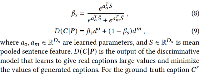
• Paper 13: Discriminative Latent Semantic Graph for Video Captioning
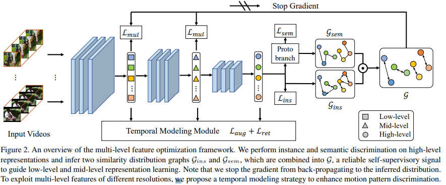
• Paper 14: Enhancing Self-supervised Video Representation Learning via Multi-level Feature Optimization
• Paper 15: Exploring simple siamese representation learning
• Paper 16: GiT: Graph Interactive Transformer for Vehicle Re-identification
• Paper 17: Graph-Time Convolutional Neural Networks
• Paper 18: Graphzoom: A multi-level spectral approach for accurate and scalable graph embedding
• Paper 19: Group Contrastive Self-Supervised Learning on Graphs
• Paper 20: Homophily outlier detection in non-IID categorical data
• Paper 21: Hyperparameter-free and Explainable Whole Graph Embedding
• Paper 22: Infograph: Unsupervised and semi-supervised graph-level representation learning via mutual information maximization
• Paper 23: Iterative graph self-distillation
• Paper 24: Learning by Aligning Videos in Time
• Paper 25: Learning graph representation by aggregating subgraphs via mutual information maximization
• Paper 26: Mile: A multi-level framework for scalable graph embedding
• Paper 27: Missing Data Estimation in Temporal Multilayer Position-aware Graph Neural Network (TMP-GNN)
• Paper 28: Multi-Level Graph Contrastive Learning
• Paper 29: Permutation-Invariant Variational Autoencoder for Graph-Level Representation Learning
• Paper 30: PiNet: Attention Pooling for Graph Classification
• Paper 31: Self-supervised Graph-level Representation Learning with Local and Global Structure
• Paper 32: Self-supervised Heterogeneous Graph Neural Network with Co-contrastive Learning
• Paper 33: SM-SGE: A Self-Supervised Multi-Scale Skeleton Graph Encoding Framework for Person Re-Identification
• Paper 34: Space-time correspondence as a contrastive random walk
• Paper 35: Spatially consistent representation learning
• Paper 36: Spatiotemporal contrastive video representation learning
• Paper 37: SportsCap: Monocular 3D Human Motion Capture and Fine-grained Understanding in Challenging Sports Videos
• Paper 38: SSAN: Separable Self-Attention Network for Video Representation Learning
• Paper 39: tdgraphembed: Temporal dynamic graph-level embedding
• Paper 40: Videomoco: Contrastive video representation learning with temporally adversarial examples
• Paper 41: Visual Relationship Forecasting in Videos
• Paper 42: Wasserstein embedding for graph learning
• Paper 43: Anomaly Detection in Video via Self-Supervised and Multi-Task Learning
• Paper 44: Exponential Moving Average Normalization for Self-supervised and Semi-supervised Learning
• Paper 45: Recognizing Actions in Videos from Unseen Viewpoints
• Paper 46: Shot Contrastive Self-Supervised Learning for Scene Boundary Detection

Paper 1: Jigsaw Clustering for Unsupervised Visual Representation Learning

Codes: https://github.com/dvlab-research/JigsawClustering

Previous pretext task

• Intra-image tasks: including colorization and jigsaw puzzle, design a transform of one image and train the network to learn the transform.
  • Since only the training batch itself is forwarded each time, they name these methods as single -batch methods.
  • Can be achieved using only one image's information, limiting the learning ability of feature extractors.
• Inter-image tasks
  • require the network to discriminate among different images.
  • Try to reduce the distance between representations of positive pairs and enlarge the distance between representations of negative samples.
  • since each training batch and its augmented version are forwarded simultaneously, methods are named as dual-batches methods.
• The way to design an efficient single-batch based method with similar performance to dual-batches methods is still an open problem.

Ideas

They propose a framework for efficient training of unsupervised models using Jigsaw clustering, which combines advantages of solving jigsaw puzzles and contrastive learning, and makes use of both intra- and inter-image information to guide feature extractor.

Jigsaw Clustering task

• Every image in a batch is split into different patches. They are randomly permuted and stitched to form a new batch for training.
• Goal : recover the disrupted parts back to the original images.
• The patches are permuted in a batch
• The network has to distinguish between different parts of one image and identifies their original positions to recover the original image from multiple montage input images.
• Why works?
  • Discriminating among different patches in one stitched image forces the model to capture instance-level information inside an image. This level of feature is missing in general in other contrastive learning methods.
  • Clustering different patches from multiple input images helps the model learn image-level features across images.
  • arranging every patch to the correct location requires detailed location information, which was considered in single-batch methods.

How?

• Batches

  

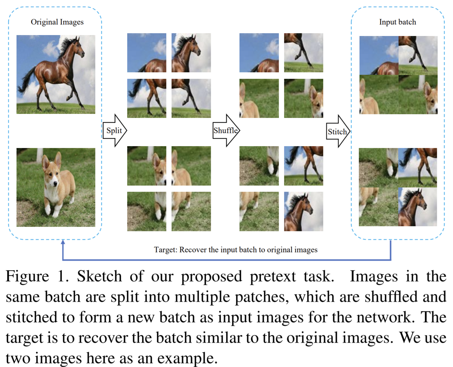
  Each batch will have \(n\) images, and after splitting (patches split in images have a level of overlap), there will be \(n\times m\times m\) patches, the patches are latterly stitched into \(n\) images. The cluster branch will cluster the \(n\times m\times m\) patches into \(n\) classes so as to define which original image that one patch comes from.

  • Using montage images as input instead of every single patch is noteworthy, since directly using small patches as input leads to the solution with only global information.
  • the input images form only one batch with the same size as the original batch, which costs half of resource during training compared with recent methods.
  • The choice of \(m\) affects the difficulty of the task. They show that \(m=2\) is good.

• Network

  • The logits is in size \(n\times m \times m\). (in location branch)

• Loss function

  • The target of clustering is pulling together objects from the same class and pushing away patches from different classes.

    

  • The loss function of location branch is simply cross-entropy loss.

  • The final objective is the weighted summation of the two losses mentioned above. But in their experiments, when the two loss are simply summed, they get the best result.

Paper 2: Self-supervised Motion Learning from Static Images

Why

• To well distinguish actions, correctly locating the prominent motion areas is of crucial importance.

Previous work

• Motion learning by architectures: two-stream networks and 3D convolutional networks. The two-stream networks extract motions representations explicitly from optical flows, while 3D structures apply convolutions on the temporal dimension or space-time cubics to extract motion cues implicitly.
• Self-supervised image representation learning: patch-based approaches , image-level pretext tasks such as image inpainting, image colorization, motion segment prediction and predicting image rotations.
• Self-supervised video representation learning: extend patch-based context prediction to spatial-temporal scenarios, e.g., spatio-temporal puzzles, video cloze procedure and frame/clip order prediction; learn representations by predicting future frames; generate supervision signals, such as speed up prediction and play back rate prediction.

How

Idea

• Learn Motion from Static Images (MoSI), take images as our data source, and generate deterministic motion patterns.
• Given the desired direction and the speed of the motions, MoSI generates pseudo motions from static images. By correctly classifying the direction and speed of the movement in the image sequence, models trained with MoSI is able to well encode motion patterns.
• Furthermore, a static mask is applied to the pseudo motion sequences. This produces inconsistent motions between the masked area and the unmasked one, which guides the network to focus on the inconsistent local motions

Motion learning from static images

Pseudo motions

• 

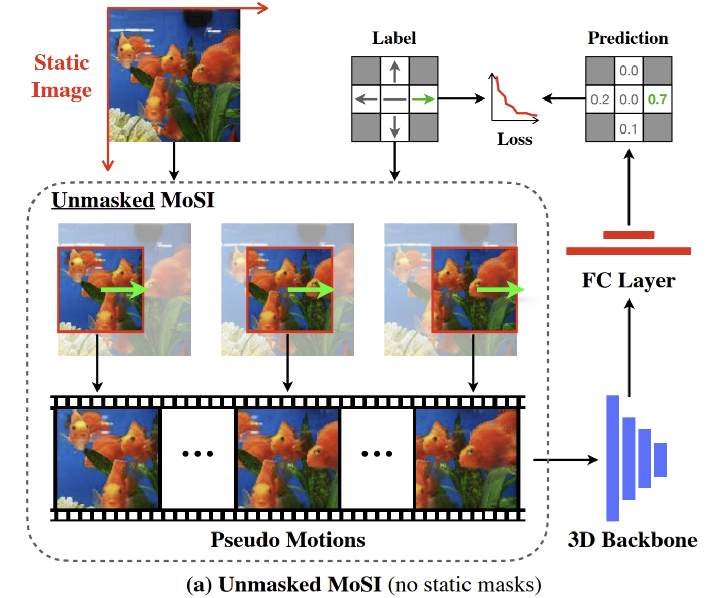
• Label pool:

  • For each label, a non-zero speed only exists on one axis.

• Pseudo motion generation

  • To generate the samples with different speeds, the moving distance from the start to the end of the Pseudo sequences are need.

    

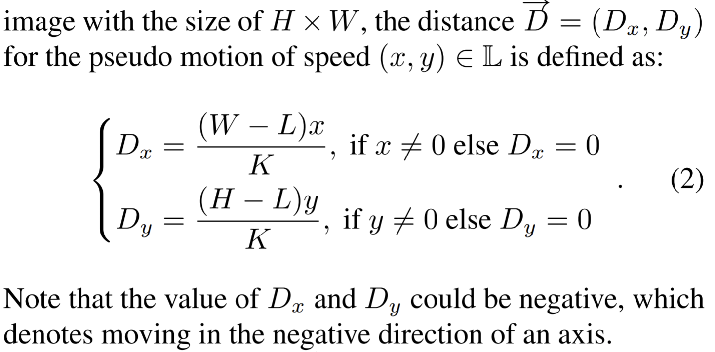
  • The start location is randomly sampled from a certain area which ensures the end location is located completely within the source image.

  • For label \((x, y) = (0, 0)\), where the sampled image sequence is static on both axis, the start location is selected from the whole image with uniform distribution.

• Classification

  • each batch contains all transformed image sequences generated from the same source image
  • The model is trained by cross entropy loss.

Static masks

• The static masks creates local motion patterns that are inconsistent with the background.
• introduce static masks as the second core component of the proposed MoSI since the model may possibly focus on just several pixels.
• 
• 
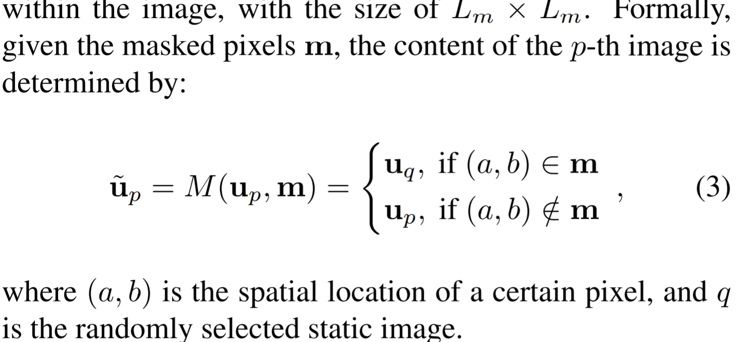
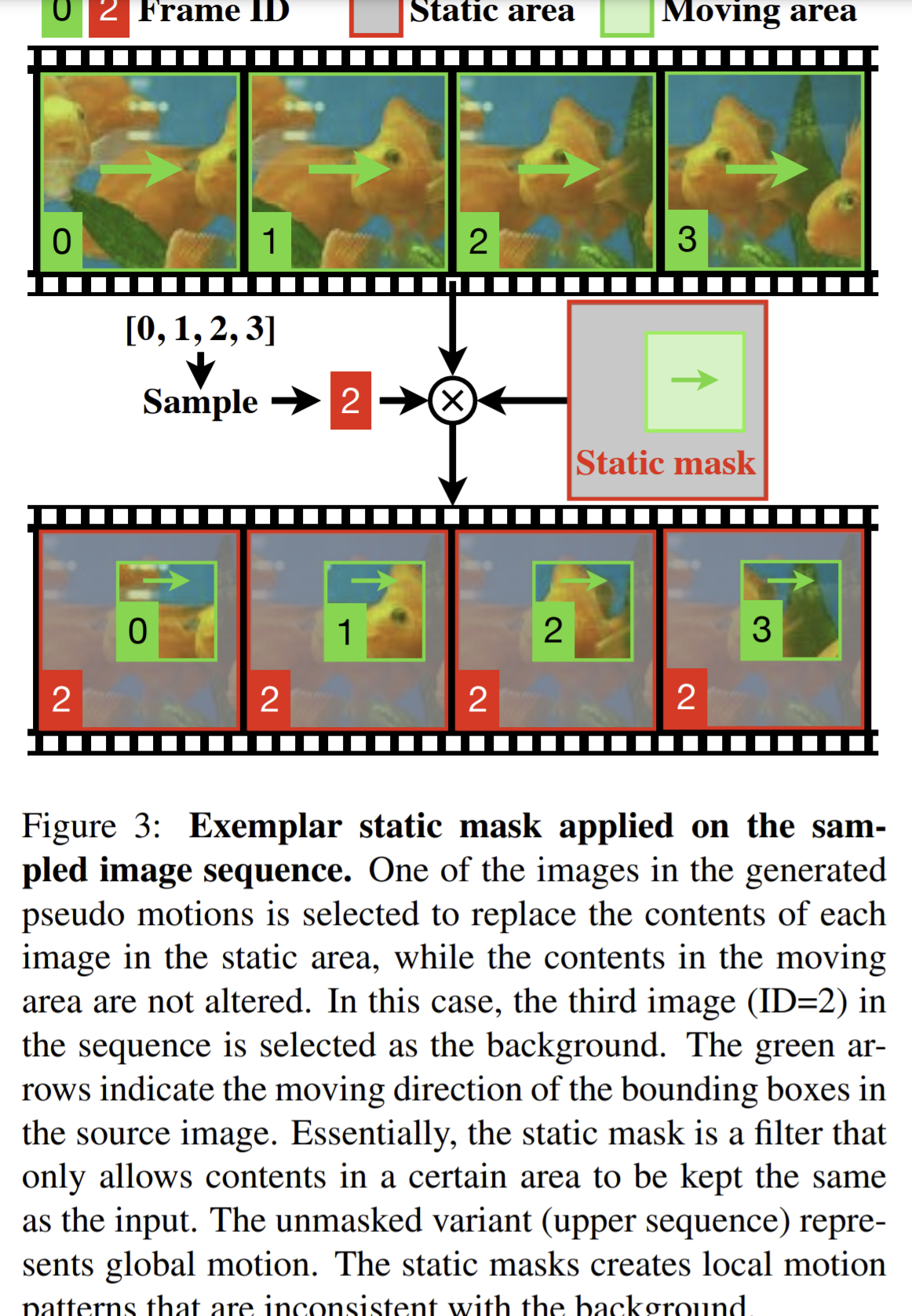
• the model is now required not only to recognize motion patterns, but also to spot where the motion is happening

Implementation

• Data preparations: the source images need to be first sampled from the videos in the video datasets.
• Augmentation: randomize the location and the size of the unmasked area. In addition, randomize the selection of the background frames in the MoSI.

Paper 3: Self-supervised Video Representation Learning by Context and Motion Decoupling

Why

• What to learn ?
  • Context representation can be used to classify certain actions, but also leads to background bias.
  • Motion representation
• Problem
  • The source of supervision: video in compressed format (such as MPEG-4) roughly decouples the context and motion information in its I-frames and motion vectors.
    • I-frames can represent relatively static and coarse-grained context information, while motion vectors depict dynamic and fine-grained movements

Previous work

• SS video representation learning
  • video specific pretext tasks: estimating video playback rates, verifying temporal order of clips, predicting video rotations, solving space-time cubic puzzles, and dense predictive coding.
  • Contrastive learning
    • clips from the same video are pulled together while clips from different videos are pushed away.
    • employ adaptive cluster assignment, where the representation and embedding clusters are simultaneously learned.
    • But they may suffer from the context bias problem.
  • mutual supervision across modalities
  • DSM: enhance the learned video representation by decoupling the scene and the motion. It simply changes the construction of positive and negative pairs in contrastive learning.
• Action recognition in compressed videos
  • Video compression techniques (e.g., H.264 and MPEG4) usually store only a few key frames completely, and reconstruct other frames using motion vectors and residual errors from the key frames.
  • Some methods directly build models on the compressed data.
    • One replace the optical flow stream in two-stream action recognition models with a motion vector stream.
    • CoViAR: use all modalities, including I-frames, motion vectors and residuals.
• Motion prediction
  • deduce the states of an object in a near future.
  • Typical models: RNNs, Transformers, and GNNs.

Goal

Design a self-supervised video representation learning method that jointly learns motion prediction and context matching.

• The context matching task aims to give the video network a rough grasp of the environment in which actions take place. It casts a NCE loss between global features of video clips and I-frames, where clips and I-frames from the same videos are pulled together, while those from different videos are pushed away.
• The motion prediction task requires the model to predict pointwise motion dynamics in a near future based on visual information of the current clip.
  • They use pointwise contrastive learning to compare predicted and real motion features at every spatial and temporal location \((x,y,t)\), which will lead to more stable pretraining and better transferring performance.
  • It works as a strong regularization for video networks, and it can also be regarded as an auxiliary task clearly improves the performance of supervised action recognition.

How

• Data: compressed videos, to be exactly, MPEG-2 Part2, where every I-frames is followed by 11 consecutive P-frames.
• Methods: context matching task for coarse-grained and relatively static context representation, and a motion prediction task for learning fine-grained and high-level motion representation.
  • context matching
    • where (video clip, I-frame) pairs from the same videos are pulled together, while pairs from different videos are pushed away
  • Motion prediction
    • 
    • Only feature points corresponding to the same video \(i\) and at the same spatial and temporal position \((x, y, t)\) are regarded as positive pairs, otherwise they are regarded as negative pairs.
    • The input and output for Transformer is considered as a 1-D sequence.
    • Some findings
      • Predicting future motion information leads to significantly better video retrieval performance compared with estimating current motion information;
      • Matching predicted and “groundtruth” motion features using the pointwise InfoNCE loss brings better results than directly estimating motion vector values;
      • Different encoder-decoder networks lead to similar results, while using Transformer performs slightly better.

Paper 4: Skip-convolutions for Efficient Video Processing

Codes: https://github.com/Qualcomm-AI-research/Skip-Conv

Why

• Leverage the large amount of redundancies in video streams and save computations
• The spiking nets is lack of efficient training algorithms
• Residual frames provide a strong prior on the relevant regions, easing the design of effective gating functions

Previous work

• Efficient video models
  • feature propagation, which computes the expensive backbone features only on key-frames.
  • interleave deep and shallow backbones between consecutive frames: methods are mostly suitable for global prediction tasks where a single prediction is made for the whole clip.
• Efficient image models: The reduction of parameter redundancies
  • model compression: Skip-Conv leverages temporal redundancies in activations.
  • conditional computations in developing efficient models for images.

Goal

To speed up any convolutional network for inference on video streams. Considering a video as a series of changes across frames and network activations, denotes as residual frames. They reformulate standard convolution to be efficiently computed over such residual frames by limiting the computation only to the regions with significant changes while skipping the others. The important residuals are learned by a gating function.

How

• The contributions
  • a simple reformulation of convolution, which computes features on highly sparse residuals instead of dense video frames
  • Two gating functions, Norm gate and Gumbel gate, to effectively decide whether to process or skip each location, where Gumbel gate is trainable.

Skip Convolutions

• Convolutions on residual frames

  • 
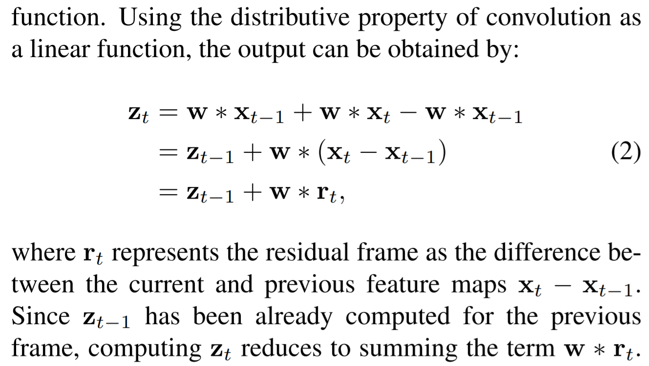
  • for every kernel support filled with zero values in \(\mathrm{r}_t\), the corresponding output will be trivially zero, and the convolution can be skipped by copying values from \(\mathrm{z}_{t−1}\) to \(\mathrm{z}_{t}\).
  • Introduce a gating function for each convolutional layer to predict a binary mask indicating which locations should be processed, and taking only \(\mathrm{r}_t\) as input. \(\mathrm{r}_t\) as input will provide a strong prior to the gating function.

• Gating functions

  • Norm gate: decides to skip a residual if its magnitude (norm) is small enough, not learnable

    • 
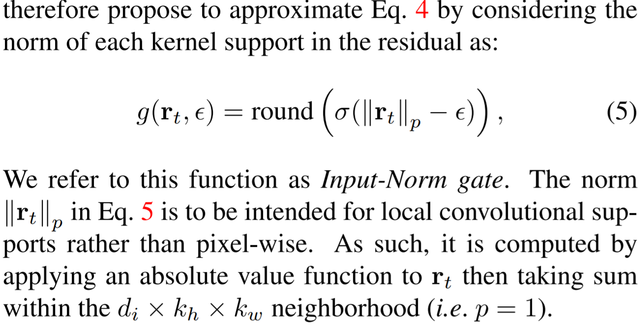
    • indicate regions that change significantly across frames, but not all changes are equally important for the final prediction.

  • Gumbel gate, trainable with the convolutional kernels.

    • A higher efficiency can be gained by introducing a higher

    • pixel-wise Bernoulli distributions by applying a sigmoid function. During training, sample binary deisions from the Bernoulli distribution.

    • Employ the Gumbel reparametrization and a straight-through gradient estimator in order to backpropagate through the sampling procedure.

    • The Gating parameters are learned jointly with all model parameters by minimizing \(\mathcal{L}_{task}+\beta \mathcal{L}_{gate}\).

    • The gating loss is defined as the average multiply-accumulate (MAC) count needed to process \(T\) consecutive frames as

      

    • train the model over a fixed-length of frames and do inference iteratively on an binary number of frames.

    • By simply adding a downsampling and an unsampling function on the predicted gates, the Skip-conv can be extended to generate structured sparsity. This structure will enable more efficient implementation with minimal effect on performance.

• Generalization and future work

  • 
  • 

Paper 5: Temporal Query Networks for Fine-grained Video Understanding

Codes: http://www.robots.ox.ac.uk/~vgg/research/tqn/

Why

• For finer-grain classification which depends on subtle differences in pose, the specific sequence, duration and number of certain subactions, it requires reasoning about events at varying temporal scales and attention to fine details.
• the constraints imposed by finite GPU memory. To overcome this, one way is to use pretrained features, but this relies on good initializations and ensures a small domain gap. Another solution focuses on extracting key frames from untrimmed videos.
• VQA (visual question and answering)
  • Have queries which attends to relevant features for predicting the answers.
  • The problem in this paper is more interested in a common set of queries shared across the whole dataset.

Goal

• Fine-grained classification of actions in untrimmed videos.

• Propose a Transformer-based video network, namely the Temporal Query Network (TQN) for fine-grained action classification, which will take a video and a predefined set of queries as input and output responses for each query, where the response is query dependent.

• The queries act as "experts" that are able to pick out from the video the temporal segments required for their response.

  • Pick out relevant temporal segments and ignore irrelevant segments.
  • Since only relevant segments will help in classification, the excessive temporal aggregation may lose the signal in the noise.

• Introduce a stochastically updated feature bank to solve memory constraints.

  • features from densely sampled contiguous temporal segments are cached over the course of training,
  • only a random subset of these features is computed online and backpropagated through in each training iteration

How

Train with weak supervision, meaning that at training time the temporal location information for the response is not proposed.

TQN

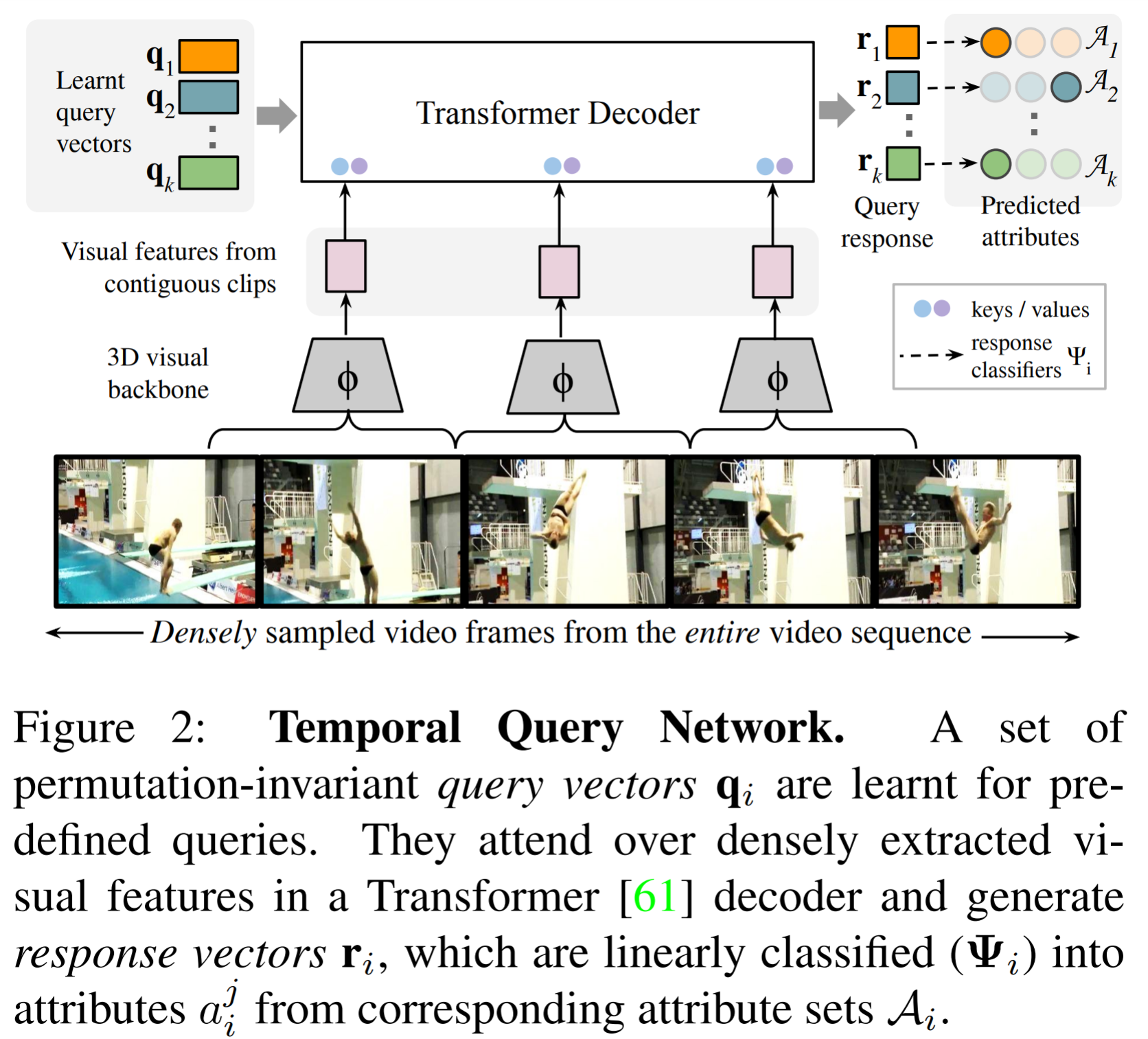
• Identifies rapidly occurring discriminative events in untrimmed videos and can be trained given only weak supervision.
• Achieves by learning a set of permutation-invariant query vectors corresponding to predefined queries about events and their attributes, which are transformed into response vectors using Transformer decoder layers attending to visual features extracted from a 3DCNN backbone.
• Given an untrimmed video, first visual features for contiguous non-overlapping clips of 8 frames are extracted using a 3D ConvNet.
• multiple layers of a parallel non-autoregressive Transformer decoder
• The training loss is a multi-task combination of individual classifier losses, which are Softmax cross-entropy, where the labels are the ground-truth attribute for the label query.

Stochastically updated feature bank

• The memory bank caches the clip-level 3DCNN visual features.
• In each training iteration, a fixed number \(n_{online}\) of randomly samples consecutive clips are forwarded through the visual encoder, while the remaining \(t-n_{online}\) clip features are retrieved from the memory bank.
• The two sets mentioned above are then combined and input into the TQN decoder for final prediction and backpropagation.
• During inference, all features are computed online without the memory bank.
• Advantages: fixed number of clips to reduce the memory price. Also enables to extend temporal context and promotes diversity in each mini-batch as multiple different videos can be included instead of just a single long video.

Factorizing categories into attribute queries

• This factorization unpacks the monolithic category labels into their semantic constituents
• The categories are factorized into multiple queries that with several attributes respectively.

Implementation

• Use S3D as visual backbone, operating on non-overlapping contiguous video clips of 8 frames.
• The decoder consists of 4 standard post-normalization Transformer decoder layers, each with 4 attention heads.
• The visual encoder is pre-trained on Kinetics-400.

Paper 6: Unsupervised disentanglement of linear-encoded facial semantics

Why

• Sampling along the linear-encoded representation vector in latent space will change the associated facial semantics accordingly.
• Current frameworks that maps a particular facial semantics to a latent representation vector relies on training offline classifiers with manually labeled datasets. Therefore they require artificially defined semantics and provide the associated labels for all facial images. If training with labeled facial semantics:
  • They demand extra effort on human annotations for each new attributes proposed
  • Each semantics is defined artificially
  • unable to give any insights on the connections among different semantics
• Previous work
  • Synthesizing faces by GAN, which changes the target attribute but keep other information ideally unchanged.
    • The comprehensive design of loss functions.
    • the involvement of additional attribute features
    • the architecture design
  • To achieve meaningful representations, one should always introduce either supervision or inductive biases to the disentanglement method
    • Inductive bias: rise from the symmetry of natural objects and the 3D graphical information.
    • Reconstruct the face images by carefully remodeling the graphics of camera principal, which makes it possible to decompose the facial images into environmental semantics and other facial semantics.
    • It's unable to generate realistic faces and perform pixel-level face editing on it.

Goal

• Photo-realistic images synthesizing, minimize the demand for human annotations
• Capture linear-encoded facial semantics.

How

With a given collection of coarsely aligned faces, a GAN is trained to mimic the overall distribution of the data. Then use the faces that the trained GAN generates as training data and trains a 3D deformable face reconstruction method. A mutual reconstruction strategy stabilizes the training significantly. Then they keep a record of the latent code from StyleGAN and apply linear regression to disentangle the target semantics in the latent space.

Decorrelating latent code in StyleGAN

• Enhance the disentangled representation by decorrelating latent codes.

  • In order to maximizes the utilization of all dimensions, they use Pearson correlation coefficient to zero and variance of all dimension.

  • Introduce decorrelation regularization via a loss function

    

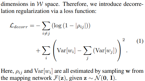
  • The mapping network is the only one to update with the new loss.

Stabilized training for 3D face reconstruction

• Use the decomposed semantics to reconstruct the original input image with the reconstruction loss

  • 
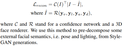
  • The 3D face reconstruction algorithm struggles to estimate the pose of profile or near-profile faces.
  • The algorithm tries to use extreme values to estimate the texture and shape of each face independently, which deviate far away from the actual texture and shape of the face. To solve this, the mutual reconstruction strategy is proposed to prevent the model from using extreme values to fit individual reconstruction, and the model learns to reconstruct faces with a minimum variance of the shape and texture among all samples.

• During training, they swap the albedo and depth map between two images with a probability \(\epsilon\) to perform the reconstruction with the alternative loss.

  

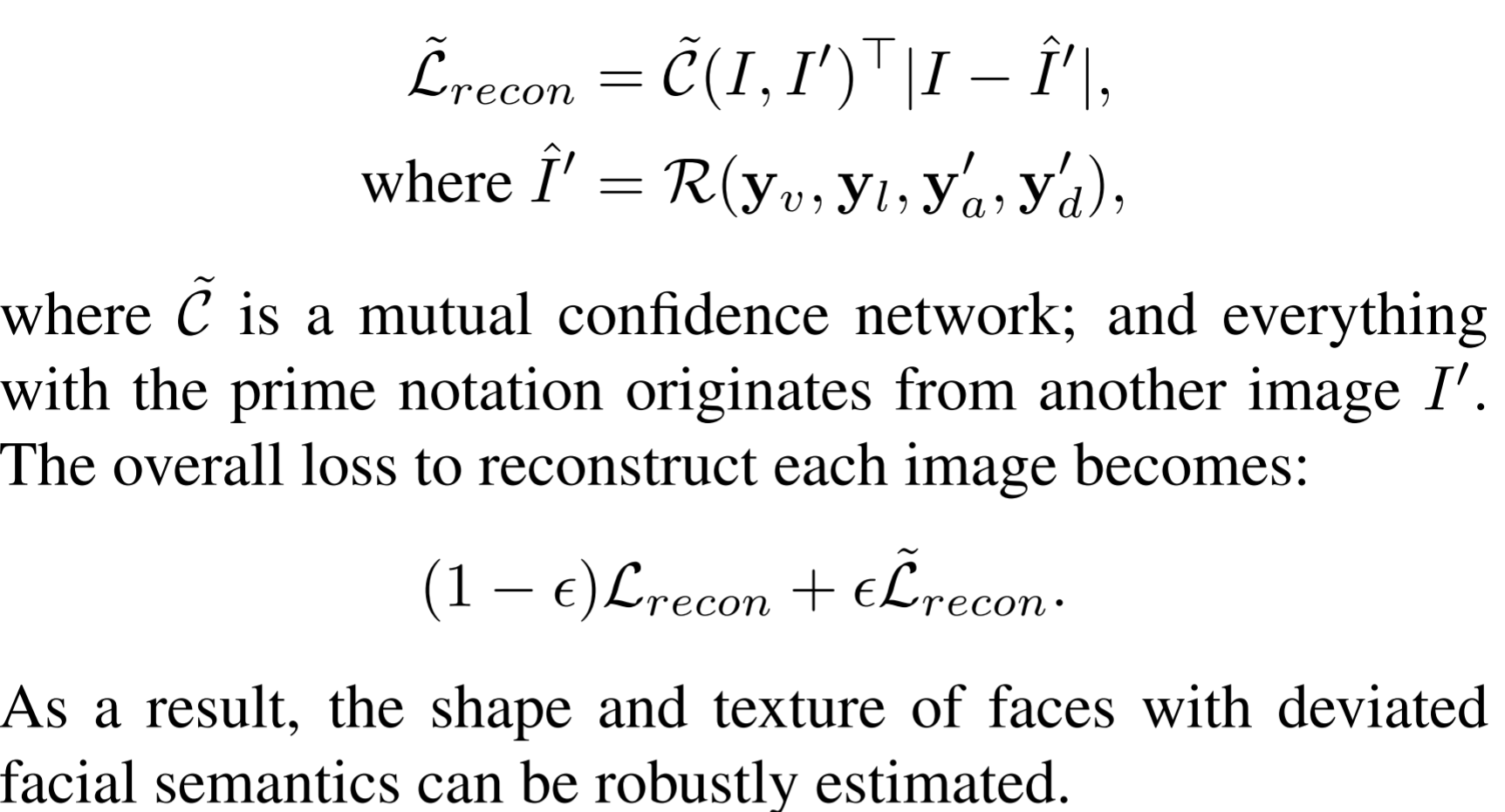
• simply concatenate the two images channel-wise as input to the confidence network

Disentangle semantics with linear regression

• The Ultimate goal of disentangling semantics is to find a vector in StyleGAN, such that it only takes control of the target semantics.
• Semantic gradient estimation
  • It's observed that with StyleGAN, many semantics can be linear-encoded. Therefore, the gradient is now independent of the input latent code.
  • 
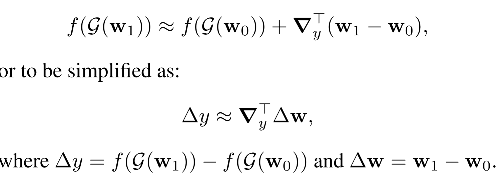
• Semantic linear regression
  • In real world scenario, the gradient is hard to estimate directly because back-propagation only captures local gradient, making it less robust to noises.
  • Propose a linear regression model to capture global linearity for gradient estimation.

Image manipulation for data augmentation

• One application is to perform data augmentation.
• By extrapolating along \(\mathrm{v}\) beyond its standard deviation, we can get samples with more extreme values for the associated semantics.

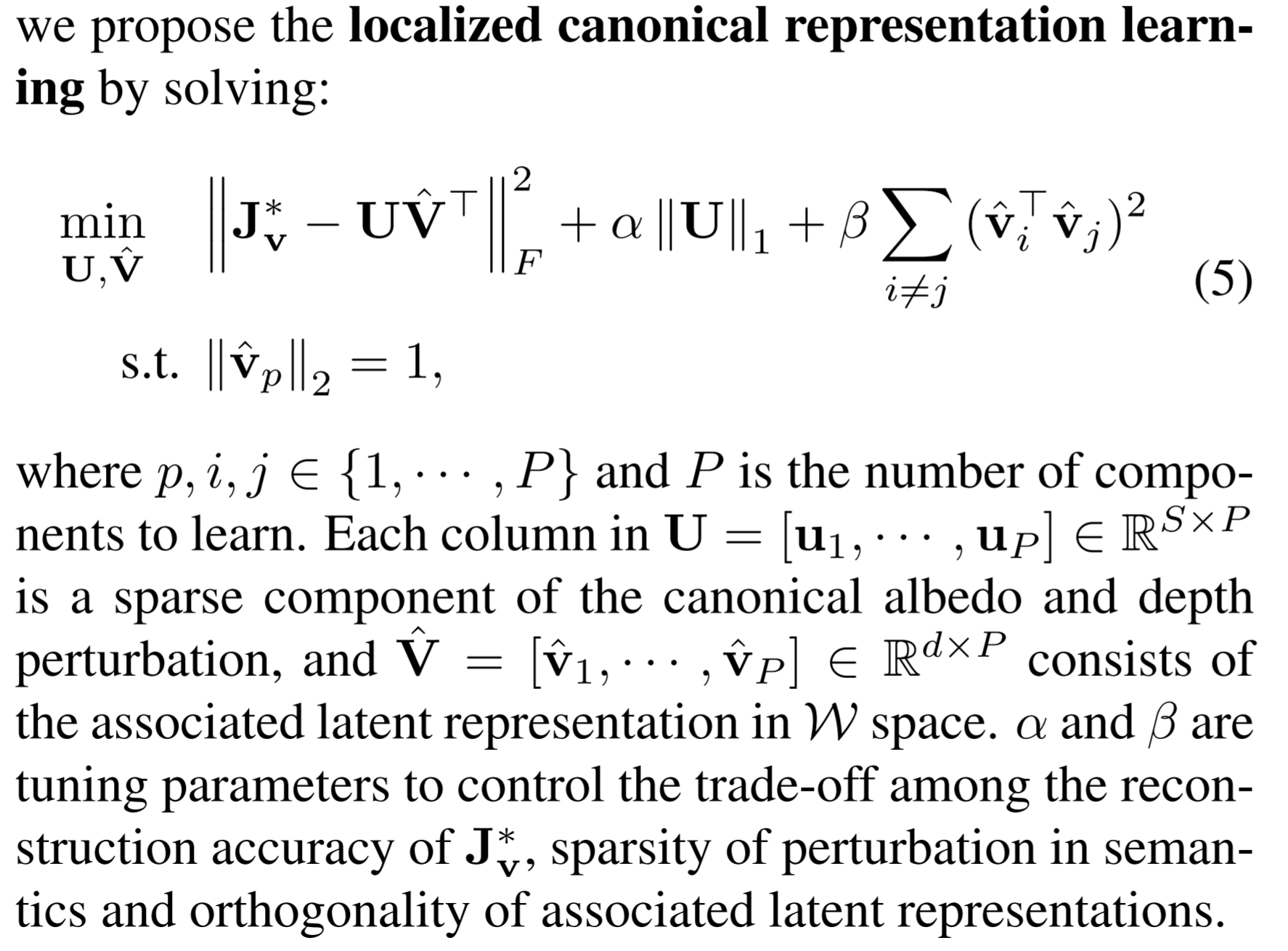
Localized representation learning

• Find the manipulation vectors \(\hat{\mathrm{v}}\) that capture interpretable combinations of pixel value variations.
• Start by defining a Jacobian matrix, which is the concatenation of all canonical pixel-level \(\mathrm{v}\).
• interpolation along \(\hat{\mathrm{v}}\) should result in significant but localized (i.e. sparse) change across the image domain.
• 

Paper 7: Bi-GCN: Binary Graph Convolutional Network

Codes: https://github.com/bywmm/Bi-GCN

Why

• The current success of GNNs is attributed to an implicit assumption that the input of GNNs contains the entire attributed graph, which will collapse or the accuracy will decrease if the entire graph is too large.
  • One intuitive solution for the problem is sampling: neighbor sampling or graph sampling. The graph sampling will sample subgraphs and can avoid neighbor explosion. But not like neighbor sampling, it cannot guarantee that each node is sampled.
    • Neighbor sampling: GraphSAGE, VRGCN
    • Sampling subgraphs: Fast-GCN, ClusterGCN, DropEdge, DropConnection, GraphSAINT for edge sampling.
  • Another solution is compressing the size of input graph data the the GNN model: such as pruning, shallow networks, designing compact layers and quantizing the parameters.
• The challenges of compressed GNN
  • The compression of the loaded data demands more attention
  • The original GNN is shallow and therefore the compression will be more difficult to be achieved.
  • Require the compressed GNNs to possess sufficient parameters for representations.

Goal

• reduce the redundancies in the node representations while maintain the principle information.

How

• Binarizes both the network parameters and input node features. The original matrices multiplications are revised to binary operations for accelerations. Design a new gradient approximation based back-propagation to train the proposed Bi-GCN.

GCN

• 

  

• Use task-dependent loss function, e.g. the cross-entropy.

Bi-GCN

Only focus on binarizing the feature extraction step, because the aggregation step possesses no learnable parameters and it only requires a few calculations. To reduce the computational complexities and accelerates the inference process, the XNOR and bit count operations are utilized.

Binarization of the feature extraction step

• Binarization of the parameters

  Each column if the parameter matrix is splitted as a bucket, and \(\alpha\) maintain the scalars for each bucket.

• Binarization of the node features

  Processed by the graph convolutional layers.

  • Split the hidden state at layer \(l\) into row buckets based on the constraints of the matrix multiplication.
  • Let \(F^{(l)}\) be the binarized buckets, the binary approximation of \(H^{(l)}\) can be obtained via
  • \(\beta\) can be considered as the node-weights for the features representations. Each element of \(F^{(l)}\) and \(B^{(l)}\) is either -1 or 1.
  • This Binarization also possesses the ability of activation, therefore the activation operations can be eliminated.

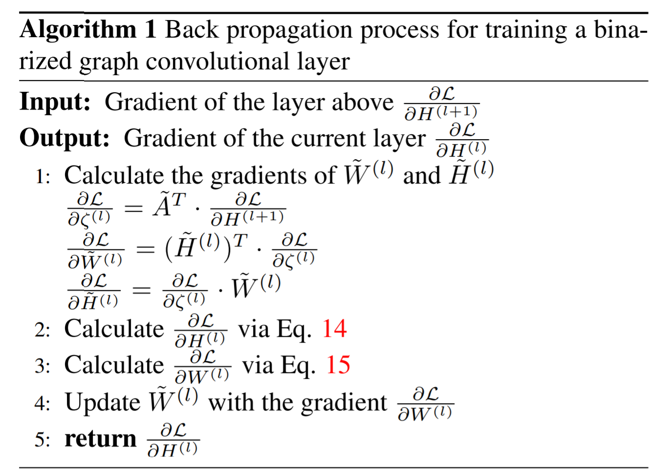
Binary gradient approximation based back propagation

Paper 8: An Attractor-Guided Neural Networks for Skeleton-Based Human Motion Prediction

Why

• Most existing methods tend to build the relations among joints, where local interactions between joint pairs are well learned. However, the global coordination of all joints, is usually weakened because it is learned from part to whole progressively and asynchronously.
• Most graphs are designed according to the kinematic structure of the human to extract motion features, but hardly do they learn the relations between spatial separated joint pairs directly.
• Except for speed, other dynamic information like accelerated speed are not counted into previous work, which ignores important motion information.
• Previous work
  • Human motion prediction
    • Many works suffer from discontinuities between the observed poses and the predicted future ones.
    • Consider global spatial and temporal features simultaneously, such as transform temporal space to trajectory space to take the global temporal information into account.
  • Joint relation modeling
    • Focus on skeletal constraints to model correlation between joints.
    • adaptive graph: the existed works weak the global coordination of all joints since they are learned from parts.
  • Dynamic representation of skeleton sequence
    • Many attempts proposed to extract enriching dynamic representation from raw data, but they only extract the dynamics from neighbor frames
    • Extract the dynamic features among frames through multiple timescale will extract more motion features.

Goal

To characterize the global motion features and thus can learn both the local and global motion features simultaneously.

Generate predicted poses through proposed framework AGN and the historical 3D skeleton-based poses.

How

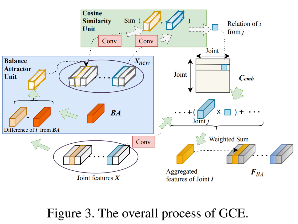
• Pipeline: A BA (balance attractor) is learned by calculating dynamic weighted aggregation of single joint feature. Then the difference between the BA and each joint feature is calculated. Later the resulting new joint features are used to calculate joints similarities to generate final joint relations.
• Framework: Attractor-Guided Neural Network, which first learn an enriching dynamic representation from raw position information adaptively through MTDE (multi-timescale dynamics extractor). Then the AJRE (attractor-based joint relation extractor) is imported , including a LIE (local interaction extractor), a GCE (global coordination extractor) and an adaptive feature fusing module.
  • AJRE: a joint relation modeling = GCE+LIE. The GCE models the global coordination of all joints, while LIE mines the local interactions between joint pairs.
  • MTDE: extract enriching dynamic information from raw input data for effective prediction.

MTDE

• A combination of different time scales motion dynamics

• Two stream, one path is the raw input poses, the other is the difference between adjacent frames in raw input. The dynamics of each joint separately is also modeled to avoid the interference of other joints.

  

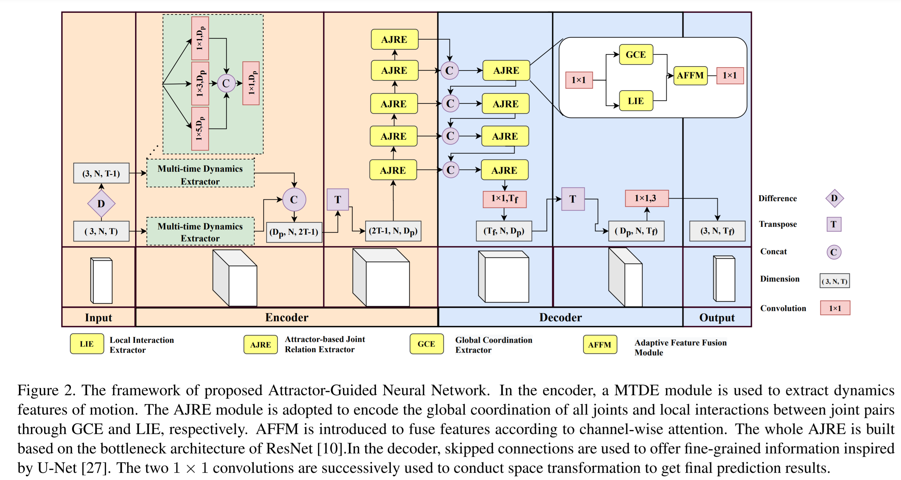
• The MTDE uses three 1DCNN but in different kernel size (5，3，1) to extract the local (joint-level) dynamics.

AJRE

• Consists of GCE and LIE to separately model global coordination of all joints and local interactions between joint pairs, and also AFFM which is used to fuse features according to channel-wise attention to improve the flexibility of joint relation modeling.
• GCE and LIE work in parallel, and they are followed by AFFM.

GCE

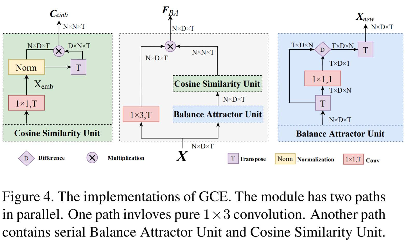
Global coordination of all joints, so they learn a medium to build new joint relations indirectly.

• BA (balance attractor unit) unit calculates all joints' aggregation to characterize the global motion features. After transpose the input features, then BA unit applies \(1\times 1\) conv to get a dynamic weighted feature aggregation of N joints features. And \(X_{new}\) is the difference between the output features of BA and the original \(X\).
• The new relations of all joints is built by the Cosine similarity unit, which measure between \(X_{new},X\). The cosine similarity between all row vector pairs to illustrate the correlation between joint pairs. The correlation matrix on each channel is calculated since each channel encodes specific spatiotemporal features and should focus on different correlations compared with other channels.

LIE

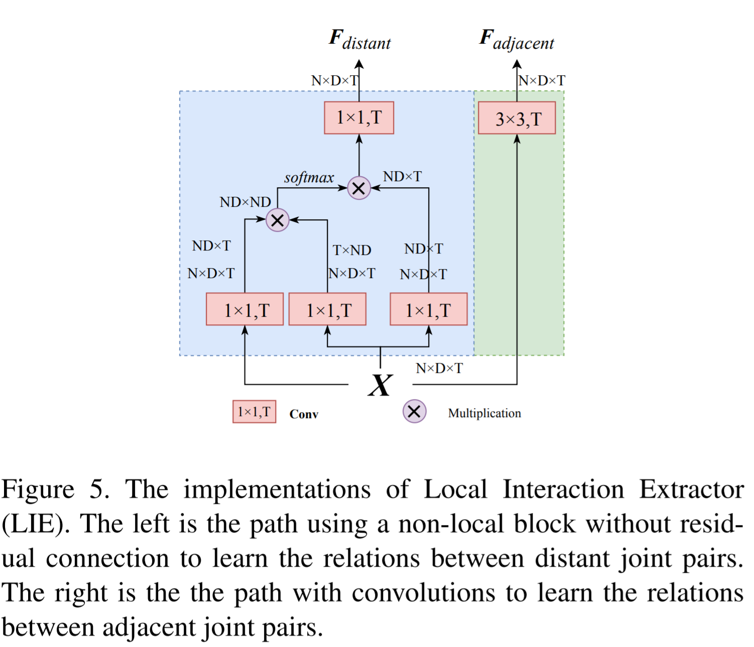
• It's used to learn local interactions between joint pairs, including adjacent and distant joints.
• To learn the relations between adjacent joint pairs, a pure \(3\times 3\) convolution is adopted. To learn the relations between distant joint pairs, the self-attention is used.

AFFM

• 
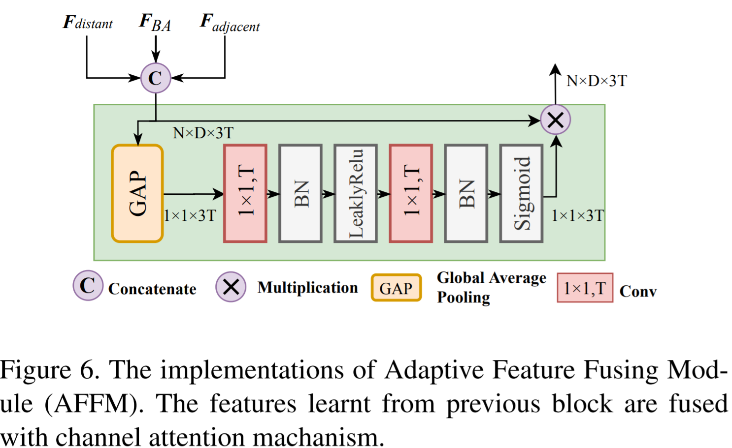
• Channel attention to fuse features adaptively and reform more reliable representation.
• After the sigmoid in the AFFM unit, the importance ratio of each channel is obtained. Then the channel-wise multiplication between ratio and raw input is done to reform features.

Paper 9: Cascade Graph Neural Networks for RGB-D Salient Object Detection

Codes: https://github.com/LA30/Cas-Gnn

Why

• How to leverage the two complementary data sources: color and depth information
• Current works either simply distill prior knowledge from the corresponding depth map for handling the RGB-image or blindly fuse color and geometric information to generate the coarse depth-aware representations, hindering the performance of RGB-D saliency detectors
• Identify saliency objects of varying shape and appearance, show robustness towards heavy occlusion, various illumination and background.
• Network cascade is an effective scheme for a variety of high-level vision applications. It will ensemble a set of models to handle challenging tasks in a coarse-to-fine or easy-to-hard manner.

Goal

Salient object detection for RGB-D images. To distill and reason the mutual benefits between the color and depth data sources through a set of cascade graphs.

Predict a saliency Map given an input image and its corresponding depth image.

How

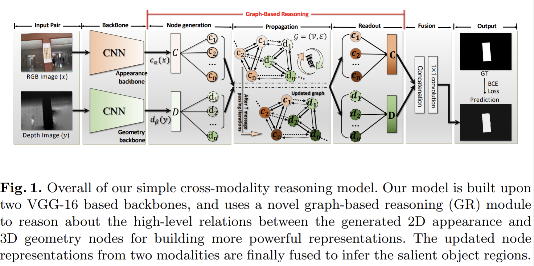
• CGR (cascade graph reasoning ) module to learn dense features, from which the saliency map can be easily inferred. It explicitly reasons about the 2D appearance and 3D geometry information for RGBD SOD.
• Each graph consists of two types of nodes, geometry nodes storing depth features and appearance nodes storing RGB-related features.
• Multiple-level graphs sequentially chained by coarsening the preceding graph into two domain-specific guidance nodes for the following cascade graph.

Cross-modality reasoning with GNNs

• Build a directed graph, where the edges connect i) the nodes from the same modality but different scales and ii) the nodes of the same scale from different modalities.
• The backbone is VGG-16 plus dilated network technique, which will extract 2D appearance representations and 3D geometry representations. They also propose a graph-based reasoning (GR) module to reason about the cross-modality, high-order relations between them.
• GRU module
  • Input 2D features and 3D features.
  • gated recurrent unit for node state updating

Cascade Graph Neural networks

• To overcome the drawbacks of independent multilevel (graph-based) reasoning, propose cascade GNNs.

• coarsening the preceding graph into two domain-specific guidance nodes for the following cascade graph to perform the joint reasoning

• The guidance nodes only deliver the guidance information, and will stay fixed during the message passing process.

• The guidance node is built by firstly concatenation and then the fusion via \(3\times 3\) convolution layer.

  

• Each guidance node propagates the guidance information to other nodes of the same domain in the graph through the attention mechanism.

• Multi-level feature fusion: The merge function is either element-wise addition or channel-wise concatenation.

Paper 10: Coarse-Fine Networks for Temporal Activity Detection in Videos

Code: https://github.com/kkahatapitiya/Coarse-Fine-Networks

Why

• One main challenge for video representation learning is capturing long-term motion from a continuous video.
• Use of frame striding or temporal pooling has been a successful strategy to cover a larger time interval without increasing the number of parameters
• Previous work
  • Action localization: temporal action localization task, which tends to annotate every frame with multiple ongoing activities. Use of sequential models such as LSTMs have been popular.
  • Dynamic sampling: selective processing of information, like spatially, temporally or spatio-temporally sampling.
• Two challenges of the network
  • how to abstract the information at a lower temporal resolution meaningfully, and
  • how to utilize the fine-grained context information effectively.

Goal

learn better video representations for long-term motion, works in multiple temporal resolutions of the input and selects frames dynamically.

How

• Grid Pool, a learned temporal downsampling layer to extract coarse features, which adaptively samples the most informative frame locations with a differentiable process.
• Multi-stage Fusion, a spatio-temporal attention mechanism to fuse a fine-grained context with the coarse features.

Grid pool

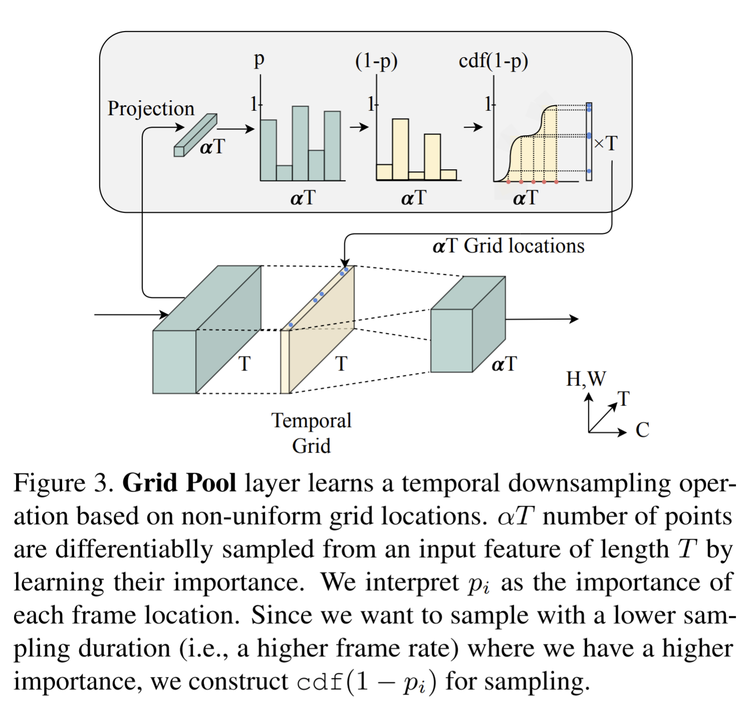
• Samples by interpolating on a non-uniform grid with learnable grid locations. The intuition comes from that sampling frames at a higher frame rate where the confidence is high and at a lower frame rate where it is low. The stride between the interpolated frame locations should be small and vice-versa.
• The confidence value is modeled as a function of the input representation.
• To get a set of \(\alpha T\) (an integer) grid locations based on confidence values, the CDF is considered.
• When a grid location is non-integer, the corresponding sampled frame is a temporal interpolation between the adjacent frames.
• A grid unpool operation is coupled with the grid locations learned by the Grid pool layer, which simply performs the inverse operation of the Grid pool. In this way, one will resamples with a low frame-rate in the regions where one used a high frame-rate in Grid pool, and vice-versa.

Multi-stage fusion

• Fuse the context from the fine stream and the coarse stream. Aims: filter out what fine-grained information should be passed down to the coarse stream, have a calibration step to align the coarse features and fine features, learn and benefit from multiple abstraction-levels of fine-grained context at each fuse-location in the coarse stream
• filtering fine-grained information: self-attention mask by processing the fine feature through a lightweight head consists of point-wise convolutional layers followed by a sigmoid non-linearity.
• Fine to coarse correspondence: use a set of temporal Gaussian distributions centered at each coarse frame location which abstract a location dependent weighted average of the fine feature.
• Multiple abstraction-levels: allow each fusion connection to look at the features from all abstraction levels by concatenating them channel-wise. The scale and shift features at each fusion location is calculated to finally fuse the features from any abstraction-levels.

Model details

• Backbone: X3D, which follows ResNet structure but designed for efficiency in video models.
• The coarse stream takes in segmented clips of \(T=64\) frames to follow the standard X3D architecture after the Grid pool later during training, while the fine stream always process the entire input clip.
• The main difference between the coarse and the fine stream is the Grid pool layer and the corresponding grid unpool operation.
• The grid pool later is placed after the 1st residual block.
• The peak magnitude of each mask is normalized to 1.
• The standard deviation \(\sigma\) is set to be \(\frac{T'}{8}\), empirically.

Paper 11: CoCoNets: Continuous Contrastive 3D Scene Representations

https://mihirp1998.github.io/project_pages/coconets/

Why

• Combine 3D voxel grids and implicit functions and learn to predict 3D scene and object 3D occupancy from a single view with unlimited spatial resolution

Goal

SSL learning of amodal 3D feature representations from RGB and RGBD posed images and videos, and finally generate the representations to help object detection, object tracks or visual correspondence.

Trained for contrastive view prediction by rendering 3D feature clouds in queried viewpoints and matching against the 3D feature point cloud predicted frim the query view.

Finally, the model forms plausible 3D completions of the scene given a single RGB-D image as input.

How

• 3d feature grids as a 3D-informed neural bottleneck for contrastive view prediction, and implicit functions for handling the resolution limitations of 3D grids.
• Propose CoCoNets (continuous contrastive 3D networks) that learns to map RGB-D images to infinite-resolution 3D scene representations by contrastively predicting views. Specifically, the model is trained to lift 2.5D images to 3D feature function grids of the scene by optimizing for view-contrastive prediction
• There are two branches in CoCoNet, one is to encode RGB-D images into a 3D feature map, and the other is to encode the RGB-D of the target viewpoint into a 3D feature cloud.
• Two branches, one adopts top-down idea which encodes the input RGB-D image and orienting the feature map to the target viewpoint, and predict the features for the target 3D points in target domain by querying, and later output a feature cloud for the target domain. The other branch is the bottom-up one, which simply encodes the target RGB-D image and predict the features for the target 3D position in target domain, obtaining the feature cloud for target domains
• The positive samples are from the target domain that works in bottom-up branch.

Result

• The scene representations learnt by CoCoNets can detect objects in 3D across large frame gaps
• Using the learnt 3D point features as initialization boosts the performance of the SOTA Deep Hough Voting detector.
• The learnt 3D feature representations can infer 6DoF alignment between the same object in different viewpoints, and across different objects of the same category.
• optimize a contrastive view prediction objective but uses a 3D girder of implicit functions as its latent bottleneck.

Paper 12: CutPaste: Self-Supervised Learning for Anomaly Detection and Localization

Codes: https://github.com/Runinho/pytorch-cutpaste

Why

• Difficult to obtain a large amount of anomalous data, and the difference between normal and anomalous patterns are often fine-grained.
• The anomaly score defined as an aggregation of pixel-wise reconstruction error or probability densities lacks to capture a high-level semantic information.
• deep one-class classifier outperforms, but most existing work focus on detecting semantic outliers, which cannot generalize well in detecting fine-grained anomalous patterns as in defet detection.
• Naively applying existed methods such as rotation prediction or contrastive learning, is sub-optimal for detecting local defects.
• Rotation and translation ect. lacks of irregularity.

Goal

• detects unknown anomalous patterns of an image without anomalous data
• Design a pretext task that can identify local irregularity.
• The pretext task is also amenable to combine with existing methods, such as transfer learning from pretrained models for better performance or patch-based models for more accurate localization

How

• Learn representations by classifying normal data from the CutPaste (data augmentation strategy that cuts an image patch at a random location of a large image). First learn SS deep representations and then build a generative one-class classifier.
• transfer learning on pretrained representations on ImageNet.
• designing a novel proxy classification task between normal training data and the ones augmented by the CutPaste. The CutPaste motivated to produce a spatial irregularity to serve as a coarse approximation of real defects.
• A two-stage framework to build an anomaly detector, where in the first stage they learn deep representations from normal data and then construct an one-class classifier using learned representations.

SSL with CutPaste

• CutPaste augmentation as follows:
  • Cut a small rectangular area of variable sizes and aspect ratios from a normal training image.
  • Optionally, we rotate or jitter pixel values in the patch.
  • Paste a patch back to an image at a random location
• 
• In practice , data augmentation or color jitter, are applied before feeding x into g or CP.

CutPaste variants

• CutPaste scar: a long-thin rectangular box filled with an image patch
• Multi-class classification: formulate a finer-grained 3-way classification task among normal, CutPaste and CutPaste-Scar by treating CutPaste variants as two separate classes.
• Similarity between CutPaste and real defects: outliers exposure. CutPaste creates examples preserving more local structures of the normal examples, while is more challenging for the model to learn to find this irregularity.
• CutPaste does look similar to some real defects.

Computing anomaly score

• A simple Gaussian density estimator whose log-density is computed as follows

  

Localization with patch representation

• CutPaste prediction is readily applicable to learn a patch representation – all we need to do at training is to crop a patch before applying CutPaste augmentation.

  

Paper 13: Discriminative Latent Semantic Graph for Video Captioning

https://github.com/baiyang4/D-LSG-Video-Caption

Why

• Key challenge of the video captioning task: no explicit mapping between video frames and captions, and the output sentence should be natural
• GNNs show particular advantages in modeling relationships between objects, but they don't jointly consider the frame-based spatial-temporal contexts in the entire video sequence
• discriminative modeling for caption generation suffers from stability issues and requires pre-trained generators.
• Traditional GNNs for video captioning cannot take adequate information into consideration, while the work of this paper (conditional graph) jointly consider objects, contexts and motion information at both region and frame levels.

Goal

• Video captioning
• Encode-decoder frameworks cannot explicitly explore the object-level interactions and frame-level information from complex spatio-temporal data to generate semantic-rich captions.
• Contributions on three key sub-tasks in video captioning
  • Enhanced object proposal: propose a novel conditional graph that can fuse spatio-temporally information into latent object proposal.
  • visual knowledge: latent proposal aggregation to dynamically extract visual words
  • sentence validation: a novel discriminative language validator
• Propose D-LSG, where the graph model for feature fusion from multiple base models, the latent semantic refers to the higher-level semantic knowledge that can be extracted from the enhanced object proposals. The discriminative module is designed as a plug-in language validator, which uses the Multimodal Low-rank Bi-linear (MLB) pooling as metrics.

How

• a semantic relevance discriminative graph based on Wasserstein gradient penalty.
• Modeled as a sequence to sequence process.

Architecture Design

• Multiple feature extraction: use 2D CNNs for appearance features and 3D CNNs for motion features. Then these two features are concatenated and apply LSTM on them.
• Enhanced object proposal: enhanced by their visual contexts of appearance and motion respectively, which result in enhanced appearance proposals and enhanced motion proposal, together these two form the enhanced object proposals.
• Visual knowledge: latent semantic proposals as \(K\) dynamic visual words, after introducing the dynamic graph built by LPA to summarize the enhanced appearance and motion features.
• Language decoder: language generation decoder will take the visual knowledge extracted by the LPA to generate captions. it consists of an attention LSTM for weighting dynamic visual words and a language LSTM for caption generation.

Latent Semantic graph

• conditional graph operation : model the complex object-level interactions and relationships, and learn informative object-level features that are in context of frame-based background information.

  • To build the graph, each region feature is regarded as a node. During message passing, the enhanced appearance proposal and object-level region features are handled with a kernel function to encode relations between them. The kernel is defined by linear functions followed by Tanh activation function.

  

• LPA

  • to further summarize the enhanced object proposals
  • propose a latent proposal aggregation method to generate visual words dynamically based on the enhanced features.
  • Introduce a set of object visual words, which means potential object candidates in the given video, and then they summarize the enhanced proposals into informative dynamic visual words.
  • 

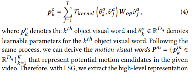
Discriminative language validation

• The module is designed to as a language validation process that encourages the generated captions to contain more informative Semantic concepts via reconstructing the visual words or knowledge based on the input sentences under the condition of corresponding true visual words encoded by LSG.
• Use WGAN-GP
• Extract sentence features from given captions by 1DCNN,
• The output of the discriminative model is weighted since sentences have different proportions of object and motion concepts
  • 
  • 

Paper 14: Enhancing Self-supervised Video Representation Learning via Multi-level Feature Optimization

https://github.com/shvdiwnkozbw/Video-Representation-via-Multi-level-Optimization

Why

• most recent works have mainly focused on high-level semantics and neglected lower-level representations and their temporal relationship
• The requirement of developing unsupervised video representation learning without resorting to manual labeling
• Drawbacks
  • previous works only explore either instance-wise or semantic-wise distribution, lacking a comprehensive perspective over both sides.
  • less effort has been placed on low-level features than high-level representations, while the former is proven critical for knowledge transfer
  • Third, directly performing temporal augmentations, e.g., shuffle and reverse, at input level instead of feature level could impair feature learning
• High-level features are more representative towards instances or semantics but less feasible towards cross-task transfer, while low-level features are transfer-friendly but lack structural information over samples.
• a line of works expanded contrastive learning pipeline to video domain
  • InfoNCE loss for dense future prediction
  • the temporal information in videos is not well leveraged
  • require a simple yet effective operation to apply temporal augmentations on extracted multi-level features

Goal

• proposes a multi-level feature optimization framework to improve the generalization and temporal modeling ability of learned video representations
• avoids forcing the backbone model to adapt to unnatural sequences which corrupts spatiotemporal statistics.
• Jointly consider the instance and semantic-wise similarity distribution to form a reliable SS signal.

How

• high-level features obtained from naive and prototypical contrastive learning are utilized to build distribution graphs
• devise a simple temporal modeling module from multi-level view features to enhance motion pattern learning.
• For low-level representation, apply temporal augmentation on multi-level features to construct contrastive pairs that have different motion patterns with the objective designed to distinguish the augmented samples and original ones. And one retrieval task is proposed to match the features in short and long time spans based on their semantic consistency.
• 

Beyond instance discrimination

• The one-hot labels in InfoNCE loss neglect the relationship between different samples. But there exist some negative samples that may share similar characteristics.
• besides instance-wise discrimination, we explicitly develop another branch on the projected high-level feature vectors for inter-sample relationship modeling.
• 
• 
• 
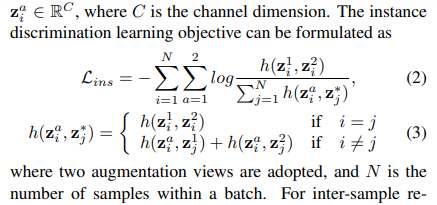
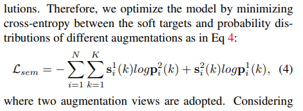
• design a queue to store the semantic-wise distributions from previous batches to ensure equal partition into K prototypes, but using only those from the current batch for gradient back-propagation
• Finally, we jointly leverage \(\mathcal{L}_{ins}\) and \(\mathcal{L}_{sem}\) to form the self-supervisory objective for high-level representations:

Graph constraint for multi-level features

• It is the lower-level features that mainly transfer from the pretrained network to downstream tasks. One can infer instance- and semantic-wise distribution from high-level features.
• Denote the instance-wise similarity distribution as a directed graph \(\mathcal{G}_{ins}\), and semantic-wise distribution as an undirected graph \(\mathcal{G}_{sem}\). Each graph contains N nodes representing N different samples within a batch, and edges indicating the relationship between each sample.
• 
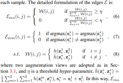
• \(\mathcal{E}_{ins}\) indicates the inferred instance-wise similarity distribution, which respects inter-sample relationship and is more realistic data distribution than one-hot encoding. \(\mathcal{E}_{sem}\) to truncate the edges between nodes of different pseudo categories.
• Jointly leverage \(\mathcal{G}_{ins}\) and \(\mathcal{G}_{sem}\) to form the combined graph \(\mathcal{G}\), whose edge weights serve as the final soft targets:
• The cross-entropy between \(\mathcal{E}\) and inferred similarity distribution to optimize lower-level features.

Temporal modeling

• Use the temporal information at diverse time scales to enhance motion pattern modeling since the features at different layers possess different temporal characteristic.

• A robust temporal model requires two aspects: semantic discrimination between different motion patters; semantic consistency under different temporal views.==> Two learning objectives

• perform temporal augmentation on multi-level features \(\mathrm{f}_r\), and then leverage a lightweight motion excitation module to extract motion enhanced feature representations

• Temporal transformations that result in semantically inconsistent motion patterns can be regarded as a negative pair of the original sample

  

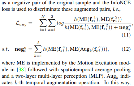
• To boost the consistency, they propose to match feature of a specific timestamp from sequences of different lengths. For one short sequence \(v_s\) that is contained in a long sequence \(v_l\), they retrieve the feature at each timestep of \(v_s\) in the feature set of \(v_l\). The feature of corresponding timestamp in \(v_l\) serves as the positive key, while others serve as negatives.

Paper 15: Exploring simple siamese representation learning

codes: https://github.com/facebookresearch/simsiam

Why

• Siamese networks are natural tools for comparing (including but not limited to “contrasting”) entities
• Recent methods define the inputs as two augmentations of one image, and maximize the similarity subject to different conditions
• An undesired trivial solution to Siamese networks is all outputs “collapsing” to a constant.
  • Methods like Contrastive learning, e.g., SimCLR etc. work to fix this.
  • Clustering is another way of avoiding constant output. While these methods do not define negative exemplars, this cluster centers can play as negative prototypes.
  • BYOL relies only on positive pairs but it does not collapse in case a momentum encoder is used. The momentum encoder is important for BYOL to avoid collapsing, and it reports failure results if removing the momentum encoder
• the weight-sharing Siamese networks can model invariance w.r.t. more complicated transformations

Goal

• report that simple Siamese networks can work surprisingly well with none of the above strategies (contrastive learning, clustering or BYOL) for preventing collapsing
• our method ( SimSiam) can be thought of as “BYOL without the momentum encoder”. Directly shares the weights between the two branches, so it can also be thought of as “SimCLR without negative pairs”, and “SwAV without online clustering”.
• SimSiam is related to each method by removing one of its core components.
• The importance of stop-gradient suggests that there should be a different underlying optimization problem that is being solved.

How

• The proposed architecture takes as input two randomly augmented views \(x_1\) and \(x_2\) from an image \(x\). The two views are processed by an encoder network \(f\) consisting of a backbone and a project MLP head. A predict MLP head is denoted as \(h\).

  

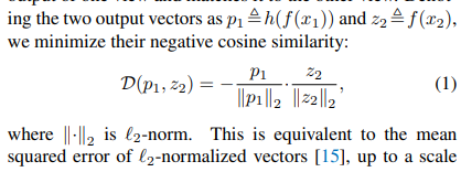
• The symmetrized loss is denoted as \(\mathcal{L}=\frac{1}{2}\mathcal{D}(p_1,p_2)+\frac{1}{2}\mathcal{D}(p_2,z_1)\). Its minimum possible value is −1.

• 

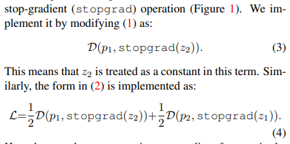
• the encoder on \(x_2\) receives no gradient from \(z_2\), but gradients from \(p_2\).

• Use SGD as optimizer, with a base \(lr=0.05\), the learning rate is \(lr\times \mathrm{BatchSize}/256\).

• Use ResNet50 as the default backbone.

• Unsupervised pretraining on the 1000-class ImageNet training set without using labels.

Paper 16: GiT: Graph Interactive Transformer for Vehicle Re-identification

Why

• Vehicle re-identification aiming to retrieve a target vehicle from non-overlapping cameras. But there are challenges
  • vehicle images of different identifications usually have similar global appearances and subtle differences in local regions
• The technologies of vehicle re-identification
  • Early methods: pure CNNs, fail to catch local information
  • Based on CNNs, cooperate part divisions (uniform spatial division suffer from partition misalignment, part detection requires a high cost of extra manual part annotations) to learn global features and local features.
  • CNNs cooperate GNNs to learn global and local features: the CNN's downsampling and convolution operations reduce the resolution of feature maps, the CNN and GNN branches are supervised with two independent loss functions and lack interaction.
  • This paper: couple global and local features via transformer and local correction graph modules.
• The advantages of transformer
  • The transformer can use multi-head attention module to capture global context information to establish long-distance dependence on global features of vehicles.
  • The multi-head attention module of transformer does not require convolution and down-sampling operations, which retain more detailed vehicle information.

Goal

Propose a graph interactive transformer (GiT) for vehicle-reidentification. Each GiT block employs a novel local correlation graph (LCG) module to extract discriminative local features within patches.

LCG Modules and transformer layers are in a coupled status.

How

• The transformer later and LCG module interact each other by skip connection when these two components work in sequence.

LCG module

• To aggregate and learn discriminative local features within every patch.

• flatten \(n\) local features \(d\) dimensions and map to \(d'\) dimensions with a trainable linear projection in every patch

• The spatial graph's edges are constructed as \(E_{v_{i,j}}=\frac{\exp (F_{cos}(v_i,v_j))}{\sum\limits_{k=1}^{n}\exp {(F_{cos}(v_i,v_k))}}\), where \(i,j\in[1，2,...,n]\). The score of the cosine distance is denoted as \(F_{cos}=\frac{v_i,v_j}{\|v_i\|\|v_j\|}\).

• To aggregate and update nodes, the aggregation node \(U\) of \(i\)-th graph is updated according as follows

  • \(U=(D^{-\frac{1}{2}}AD^{-\frac{1}{2}}X_i)\cdot W\),

  • Then \(U\) is processed non-linearly as

    \(O=GELU(LN(U))\), where GELU represents the gaussian error linear units and LN denotes the layer normalization.

Transformer layer

• Model the global features between the different patches.
• Patches are the input for multi-head attention layer
• Later, the output from the attention layer is normalized and then processed by MLP.

Graph interactive Transformer

• Each GiT block consists of a LCG module and a Transformer layer.

Loss function design

• The proposed GiT's total loss function is

  \(L_{total}=\alpha L_{CE}+\beta L_{Triplet}\), where \(L_{CE}\) denote cross-entropy loss, and \(L_T\) denotes triplet loss.

• The \(L_{CE}\) formulates the cross-entropy of each patch's label

• The triplet loss is

  

Paper 17: Graph-Time Convolutional Neural Networks

Codes: https://github.com/gtcnnpaper/DSLW-Code

Why

• The key for learning on multivariate temporal data is to embed spatiotemporal relations into into its inner-working mechanism.
• Spatiotemporal graph-base models
  • Hybrid: combine learning algorithms developed separately for the graph domain and the temporal domain
    • Such as a temporal RNN, CNN
    • their spatial and temporal blocks are modular and can be implemented efficiently
    • unclear how to best interleave these blocks for learning from spatiotemporal relationships
  • Fused
    • force the graph structure into conventional spatiotemporal solutions and provide a single strategy to jointly capture the spatiotemporal relationships.
    • substitute the parameter matrices in these models with graph convolutional filters
    • fused models capture naturally these relationships as they have graph-time dependent inner-working mechanisms.

Goal

• Represent spatiotemporal relations through product graphs and develop a first principle graph-time convolutional neural network (GTCNN).
• For multivariate temporal data such as sensor or social networks

How

• Each layer consists of a graph-time convolutional module, a graphtime pooling module, and a nonlinearity.
• The product graph itself is parametric to learn the spatiotemporal coupling
• The zero-pad pooling preserves the spatial graph while reducing the number of active noes and parameters

Signals over product graphs

• Two graphs:

  • Spatial graph \(\mathcal{G}\), consider the original sensor network, each node has a time sequence
  • Temporal graph \(\mathcal{G}_T\): for each node, there is a line graph that take each timestep as a node.

• Given graphs \(\mathcal{G}\) and \(\mathcal{G}_T\) , we can capture the spatiotemporal relations in \(\mathrm{X}\) through the product graph \(\mathcal{G}_\diamond = \mathcal{G}_T\times \mathcal{G}=(\mathcal{V}_\diamond,\mathcal{E}_\diamond)\) , where the vertex set \(\mathcal{V}_\diamond = \mathcal{V}_T \times \mathcal{V}\) is the Kronecker product between \(\mathcal{V}_T\) and \(\mathcal{V}\).

• Product graphs

  

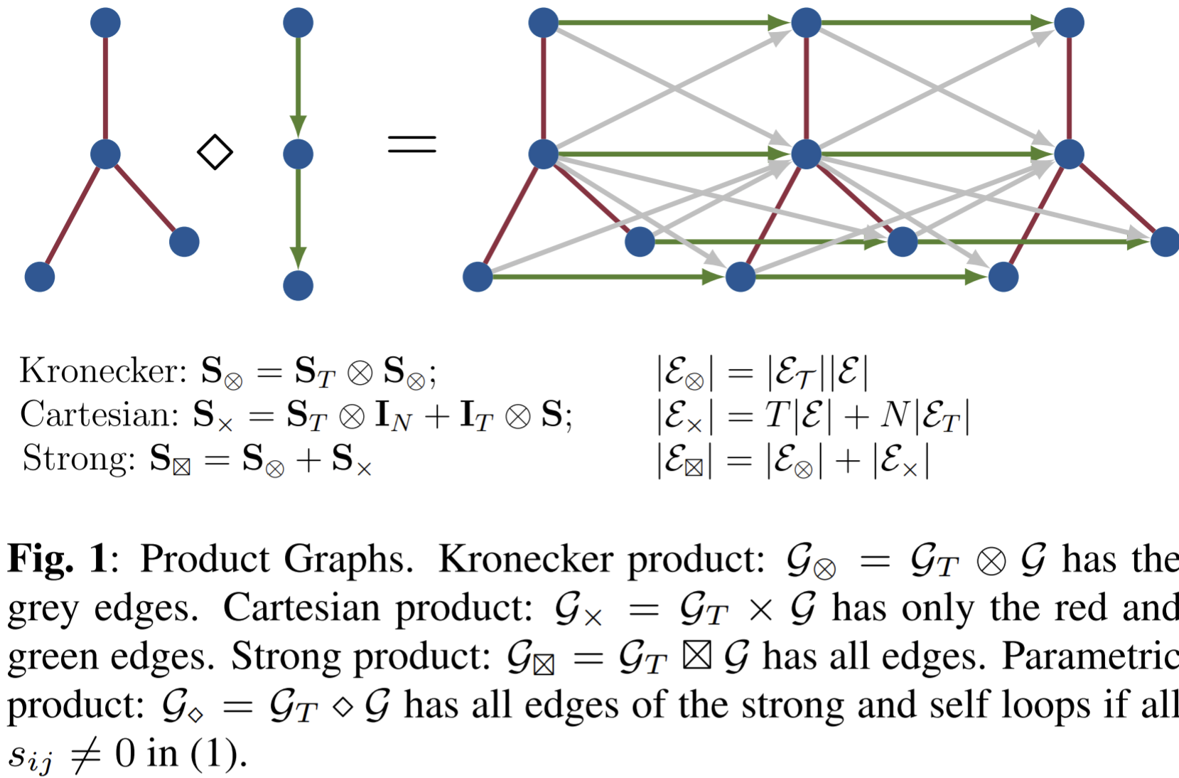
  • The Kronecher product preserves the relations between different nodes along temporal dimension. The 1st node at the 1st timestep have influences for the 2nd node at the 2nd timestep. And the influence is bidirectional.
  • The cartesian product preserves the original spatial infromation and the temporal evolution on each node's temporal dimension.

• Goal: to learn spatiotemporal representations in a form akin to temporal or graph CNNs.

Graph-time CNNs

• A compositional architecture of \(L\) layers each having a graph-time convolutional module, a graph-time pooling module and a nonlinearity.
• 
• at convolutions allow for effective parameter sharing, inductive learning, and efficient implementation, while zero-pad pooling and pointwise nonlinearities make the architecture independent from graph-reduction techniques or other modules.
• Graph-time convolutional filtering
  • The graph-time convolutional filter aggregates at the space-time location \((i, t)\) information from space-time neighbors that are up to \(K\) hops away over the product graph \(\mathcal{G}_\diamond\).
  • 
  • Implement it recursively, and expand all polynomials of order \(k\). Then the computational cost is liner in the product graph dimensions.
• Graph-time pooling: The pooling approach has three steps: i) summarization; ii) slicing; iii) downsampling
  • Summarization: up to \(\alpha_l\) hops away for each node . Use mean or max function.
    • Summarization is an implicit low-pass operation and the type of product graph has an impact on its severit
  • Slicing: reduces the dimensionality across the temporal dimension.
  • Downsampling: reduces the number of active nodes across the spatial dimension from \(N_{l-1}\) to \(N_l\) without modifying the underlying spatial graph.

Paper 18: Graphzoom: A multi-level spectral approach for accurate and scalable graph embedding

Codes: https://github.com/cornell-zhang/GraphZoom

Why

• Challenges
  • existing graph embedding models either fail to incorporate node attribute information during training or suffer from node attribute noise, which compromises the accuracy
  • few of them scale to large graphs due to their high computational complexity and memory usage
• Graph embedding techniques
  • Random-walk-based embedding algorithms
    • embed a graph based on its topology without incorporating node attribute information==> limits the embedding power
    • GCN with the basic notion that node embeddings should be smoothed over the entire graph and so can leverage both topology and node attribute information.==> But may suffer from high-frenquency noise in the inital node features.
• Only one of the solution for increasing the accuracy or improving the scalability of graph embedding methods is well-handeled. Not all of them
• Previous work
  • Multi-level graph embedding: GraphZoom is motivated by theoretical results in spectral graph embedding.
  • Graph filtering: GCN model implicitly exploits graph filter to remove high-frequency noise from the node feature matrix. In GraphZoom we adopt graph filter to properly smooth the intermediate embedding results during the iterative refinement step.

Goal

• Propose GraphZoom, a multi-level framework for improving both accuracy and scalability of unsupervised graph embedding algorithms.

How

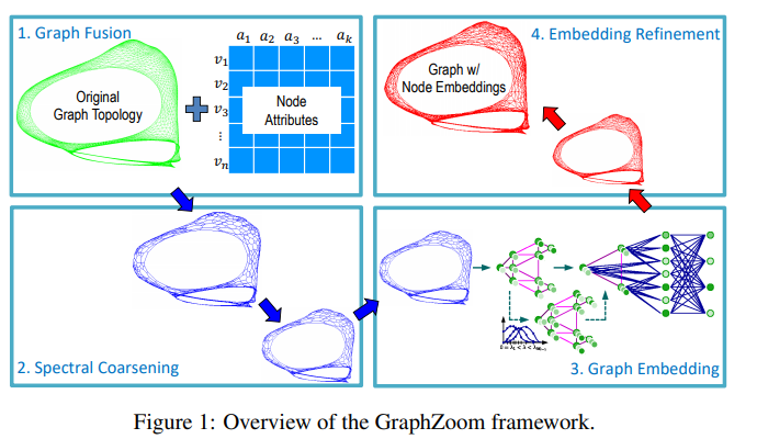
• GraphZoom consists of four major kernels: (1) graph fusion, (2) spectral graph coarsening, (3) graph embedding, and (4) embedding refinement.
  • The graph fusion kernel first converts the node feature matrix into a feature graph and then fuses it with the original topology graph.
  • Spectral graph coarsening produces a series of successively coarsened graphs by merging nodes based on their spectral similarities.
  • During the graph embedding step, any of the existing unsupervised graph embedding techniques can be applied to obtain node embeddings for the graph at the coarsest level.
  • Embedding refinement is then employed to refine the embeddings back to the original graph by applying a proper graph filter to ensure embeddings are smoothed over the graph.

Graph Fusion

• To construct a weighted graph that has the same number of nodes as the original graph but potentially different set of edges (weights) that encapsulate the original graph topology as well as node attribute information
• Firstly generate a KNN graph based on the \(\ell^2-norm\) distance between the attribute vectors of each node pair so to convert initial attribute matrix \(X\) into a weighted node attribute graph.
• To implement in a linear cost, they start with coarsening the original graph \(\mathcal{G}\) to obtain a substantially reduced graph that has much fewer nodes with an \(\mathcal{O}(|\mathcal{E}|)\) , similar as to spectral graph clustering to group nodes into clusters of high conductance. After the attribute graph is formed, we assign a weight to each edge based on the cosine similarity between the attribute vectors of the two incident nodes. Finally, we can construct the fused graph by combining the topology graph and the attribute graph using a weighted sum: \(\mathrm{A}_{fusion}=\mathrm{A}_{topo}+\beta \mathrm{A}_{feat}\).

Spectral coarsening

• For graph coarsening via global spectral embedding: calculating eigenvectors of the original gragh Laplacian is very costly. To eliminate the cost, they propose a method for graph coarsening via local spectral embedding.
  • The analogies between the traditional signal processing (Fourier analysis) and graph signal processing.
    • The signals at different time points in classical Fourier analysis correspond to the signals at different nodes in an undirected graph;
    • The more slowly oscillating functions in time domain correspond to the graph Laplacian eigenvectors associated with lower eigenvalues or the more slowly varying (smoother) components across the graph.
  • apply the simple smoothing (low-pass graph filtering) function to \(k\) random vectors to obtain smoothed vectors for \(k\)-dimensional graph embedding, which can be achieved in linear time.
• We adopt low-pass graph filters to quickly filter out the high-frequency components of the random graph signal or the eigenvectors corresponding to high eigenvalues of the graph Laplacian, and then get the smoothed vectors in \(T\) (initial random vectors).
• The aggregation scheme:
• Once the aggregation scheme is defined, the coarsening in multilevel is formed as a set of graph mapping matrices.

Graph embedding

Just obtain embedding according to the previously defined formulas.

Embedding refinement

• To get the embedding vectors for the original graph eventually. It's kind of like remapping the graph from the coarsest level to the finest level.
• The refinement process is motivated by Tikhonov regularization to smooth the node embedding over the graph by minimizing \(\min\limits_{E_i}\{\|E_i-\hat{E}_i\|^2_2+tr(E_i^\top L_iE_i)\}\), where \(L_i\) and \(E_i\) are the normalized Laplacian matrix and mapped embedding matrix of the graph at the \(i\)-th coarsening level, respectively. The solving the equation, the refined embedding matrix of edges are solved.
• To solve the equation efficiently , they work in spectral domain, and approximate the graph filter by it first-order Taylor expansion.
• 

Paper 19: Group Contrastive Self-Supervised Learning on Graphs

Why

• Capability : Contrasting graphs in multiple subspaces enables graph encoders to capture more abundant characteristics.
• CL methods train models on pretext tasks that encode the agreement between two views of representations. These two views can be global-local pairs or differently transformed graph data. The learning goal is to make these two-view representations similar if they are from the same graph and dissimilar if they are from different graphs.
• The idea of using groups has been shown to be effective in the image domain.

Goal

• Study SSL on graphs by contrastive learning.
• Propose a group contrastive learning framework. Embed the given graph into multiple subspaces, of which each representation is prompted to encode specific characteristics of graphs.
• Further develop an attention-based representor function to compute representations. Develop principled objectives that enable us to capture the relations among both intra-space and inter-space representations in groups.

How

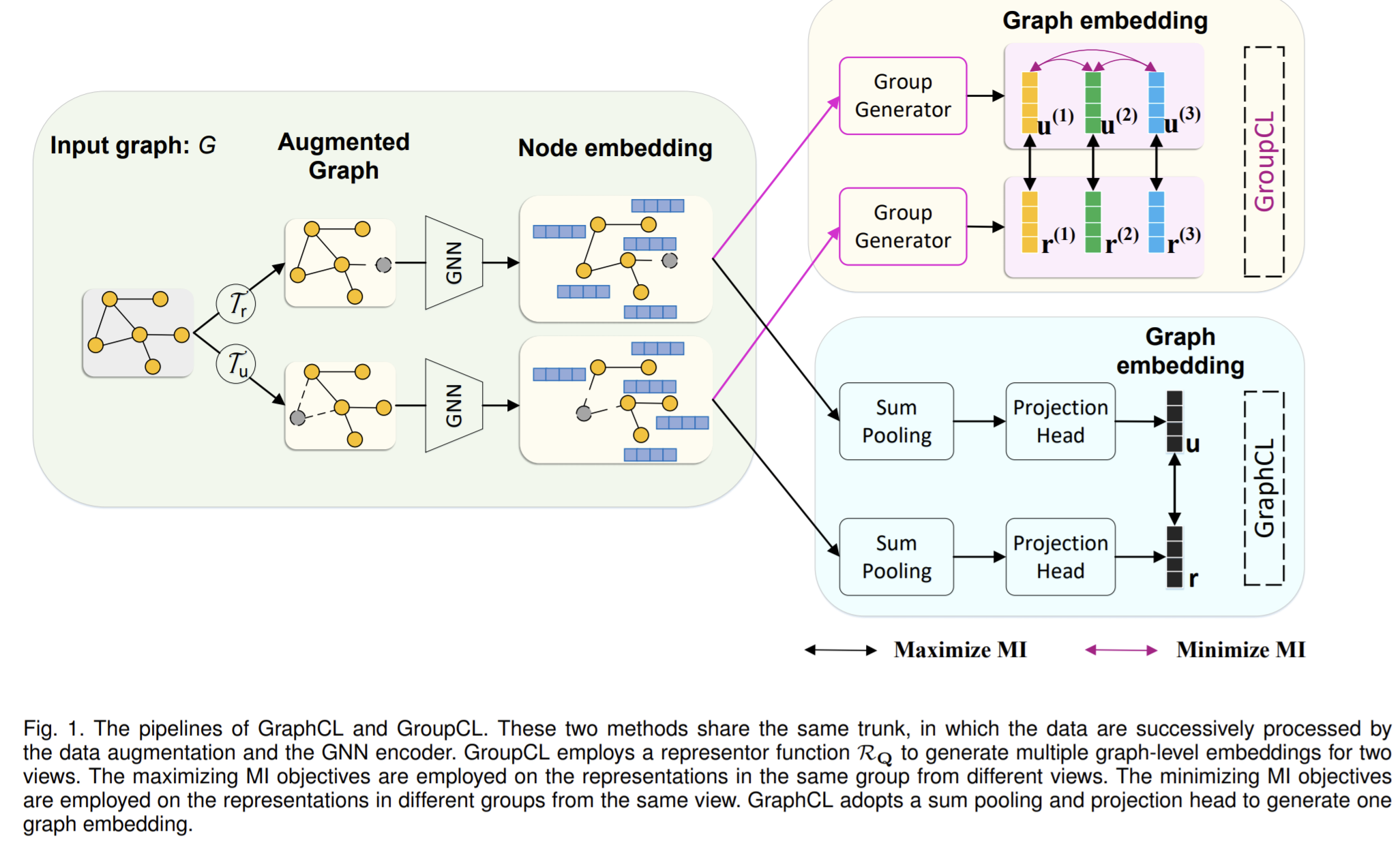
• refer to a group as a set of representations of different graph views within the same subspace
• propose to maximize the MI between two views of representations in the same group while minimizing the MI between the representations of one view across different groups.
• a graph-level encoder usually consists of a node encoder which computes the node embedding matrix and a readout function summarize the mdoe embeddigs into the desired graph-level embedding.

The proposed group contrastive learning framework

• To build two views and their corresponding multiple graph-level representations. The used GNN encoder can be the same, or one can just duplicate the calculated representation for \(p\) times. Then for view \(u,r\), they can be combined into \(p\) pairs which are cross-view pairs and two groups that each group from one specific view.
• So for two views: the main view \(u\), and auxiliary view \(r\), there are in total two encoders which are parameterized by \(\theta, \phi\) respectively.

Intra-space objective function

• For the intra-space objective, they seek to maximize the mutual information between representations of two views within each group. The optimization is done based on paramters \(\theta,\phi\).
• To implement, maximizes the MI's lower-bound. Precisely, they adopt the Jensen-Shannon estimator of MI, and the disciriminator is the dot product between two representations.

Inter-space objective function

• Constraint the pairwise relation across different groups of the same view to enforce the diversity of inter-space. They employ an inter-space optimization objective based on mutual information minimization.
• To minimize the MI, we introduce an upper bound of MI as an efficient estimation, based on the contrastive log-ratio upper bound: . To solve the key challenge of modeling \(P(y|x)\), there are two approaches based on whether the same dimensions of \(x\) and \(y\) correspond to each other across different representations. Suppose the distribution \(y\) conditional on \(x\) is subject to a Gaussian distribution.
  • Non-parameterized estimation
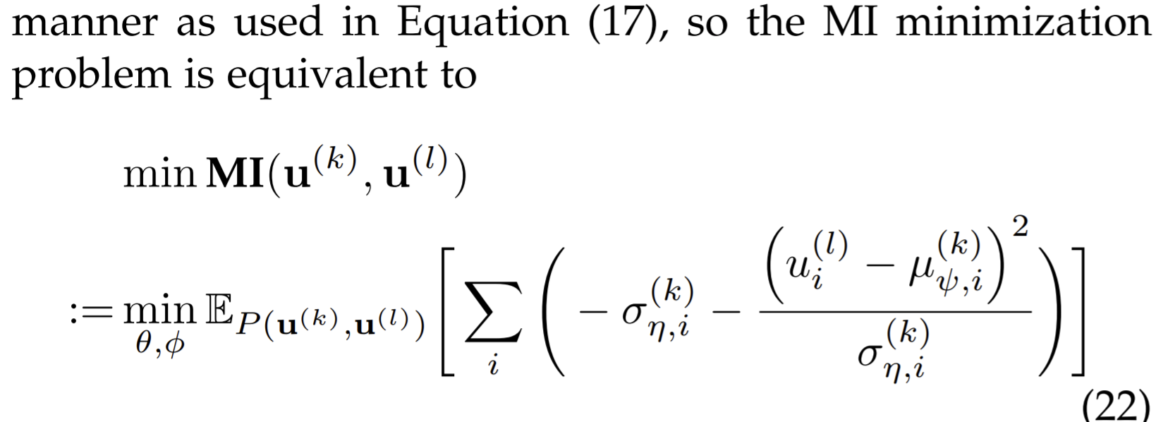
    • Assume \(\mathbb{E}[y|x]=x\), and the variance \(\Sigma\) is a diagonal matrix with the same values on its diagonal. Then after deduction, the goal minimizing CLUB is equivalent to minimize
    • This goal enlarges the agreement between \(\mathrm{u}^{(k)},\mathrm{u}^{(l)}\), under the joint distribution so to keep the diversity among one group.
  • Parameterized estimation
    • When there is no correspondence between dimensions of \(x,y\).
    • Via a parameterized variational distribution. Concretely, they use two independent MLP to generate the mean and variance respectively.
    • 

The overall objective function

• Combine the intra-space and the inter-space objectives together.
• Either optimize based on non-parameterized way or parameterized way.

GroupCL: GraphCL with Group Contrast

• the generation of multiple representations shares the same node encoder and envolves a parameterized representor function that computes multiple graph representations from node embeddings of a given graph.
• For view \(u\), GroupCL performs a random data augmentation on the input graph to generate the view data, and then use encoder to encode each nodes of the view data into node embeddings \(\mathrm{U}\). Given \(\mathrm{U}\), use attention to capture the information from different node combinations where each graph representation depends greatly on the heavily attended nodes with respect to different queries, and thus propose the representor function.
• the multiple representations are prompted to focus on different and informative combinations of nodes and thereupon encode different subgraph patterns.

GraphIG: InfoGraph with Group Contrast

• In InfoGraph, view \(u,r\) are the graph-level embedding an the node-level embedding, respectively.
• In view \(u\), the encoder GNN and representor function \(\mathcal{R}_Q\) is similar as GroupCL.
• In view \(r\), they generate the node embeddings through encder GNN and duplicate them for \(p\) times to obtain \(p\) representations.

Paper 20: Homophily outlier detection in non-IID categorical data

 Will be completed later.

Why

Goal

• identify outliers in categorical data by capturing non-IID outlier factors

How

• first defines and incorporates distribution-sensitive outlier factors and their interdependence into a value-value graph-based representation. Then model an outlierness propagation process in the value graph to learn the outlierness of feature values.

Paper 21: Hyperparameter-free and Explainable Whole Graph Embedding

Codes: https://github.com/HW-HaoWang/DHC-E

Why

• most node embedding or whole graph embedding methods suffer from the problem of having more sophisticated methodology, hyperparameter optimization, and low explainability.
• Previous work
  • Before 2000, traditional methods like PCA, LDS are linear, which cannot handle the nonlinear relationships within datasets properly.
  • Around 2000, like IsoMap and LLE (Laplacian eigenmaps) are manifold.
  • From practical view, like word2vec is popular.
• Whole graph embedding methods: previously they are mathematically intractable, sophisticated, and challenging to interpret, and suffer hyperparameter selection problems in comparing different graphs.
  • FGSD (family of graph spectral distances): calculate the Moore-Penrose spectrum of the normalized Laplacian and use the histogram of the spectral features as a whole graph representation.
  • Graph2vec: unsupervised, derive fixed-length task-agnostic embedding of graphs
  • NetLSD (Network Laplacian Spectral Descriptor) : calculate the heat kernel trace of the normalized Laplacian matrix over a vector of time scales.
  • IGE (Invariant graph embedding): compute a mixture of spectral and noes embedding based features and pool node feature embedding to create graph descriptor.
  • GL2vec: complement the edge label information or the structural information .

Goal

• This paper only considers unweighted and undirected graphs with no self-loops or multiple edges.
• Propose a hyperparameter free, extensible, and explainable whole graph embedding method, combining the DHC (Degree, H-index and Coreness) theorem and Shannon Entropy (E), abbreviated as DHC-E.
• The new whole graph embedding scheme can obtain a trade-off between simplicity and quality under supervised classification learning tasks, using molecular, social, and brain networks. In addition, the proposed approach has a good performance in lower dimensional graph visualization

How

• DHC-E can be regarded as an adaptive and self-converging system that depicts the information of complex systems from the fine-grained to coarse-scale.
• Assume that different networks have different convergence steps and each iteration of H-index sequences encodes information that can distinguish the network’s properties.
• metrics for vital node identification
  • Degree
  • H-index: The h-index of a node in the graph is defined as the maximum value \(h\) such that there exist at least \(h\) neighbors who have a degree no less than \(h\). The H-index of every node can be updated based on the previous H-indices of neighbors following the same procedure.
  • Coreness: take the location of a node in the graph to measure its influence based on the \(k\)-core decomposition process. A larger coreness of a noes indicate that it is located more centrally in the graph.

DHC-entropy

• DHC theorem proves that each nodal H-index sequence eventually converges to the nodal coreness.

• The zero-order H-index of every node is initialized to its degree, as shown in the initial state. The following updated states can be calculated by the DHC theorem

• Combining Shannon entropy and DHC theorem:

  • Problems: : (1) How to extract and integrate the information generated from the DHC updating process (i.e., the H-index sequences of all nodes) to construct whole graph embedding; (2) How to unify and align the whole graph embedding with different dimensions.
  • In the \(m\)-th iteration, for the H-indices, calculate the probability distribution of each node's H-index, and then take the probability distribution to calculate Shannon-entropy, so to quantify the uncertainty of the graph in this state.
  • To align, for one graph set with different subgraphs to have same dimension of embeddings so as to perform whole graph embedding aggregation, the key is to keep the number of H-indices of each subgraphs to be the same. They propose to expand those with smaller H-indices to be expanded with their last element.

• The DHC-E algorithm

  

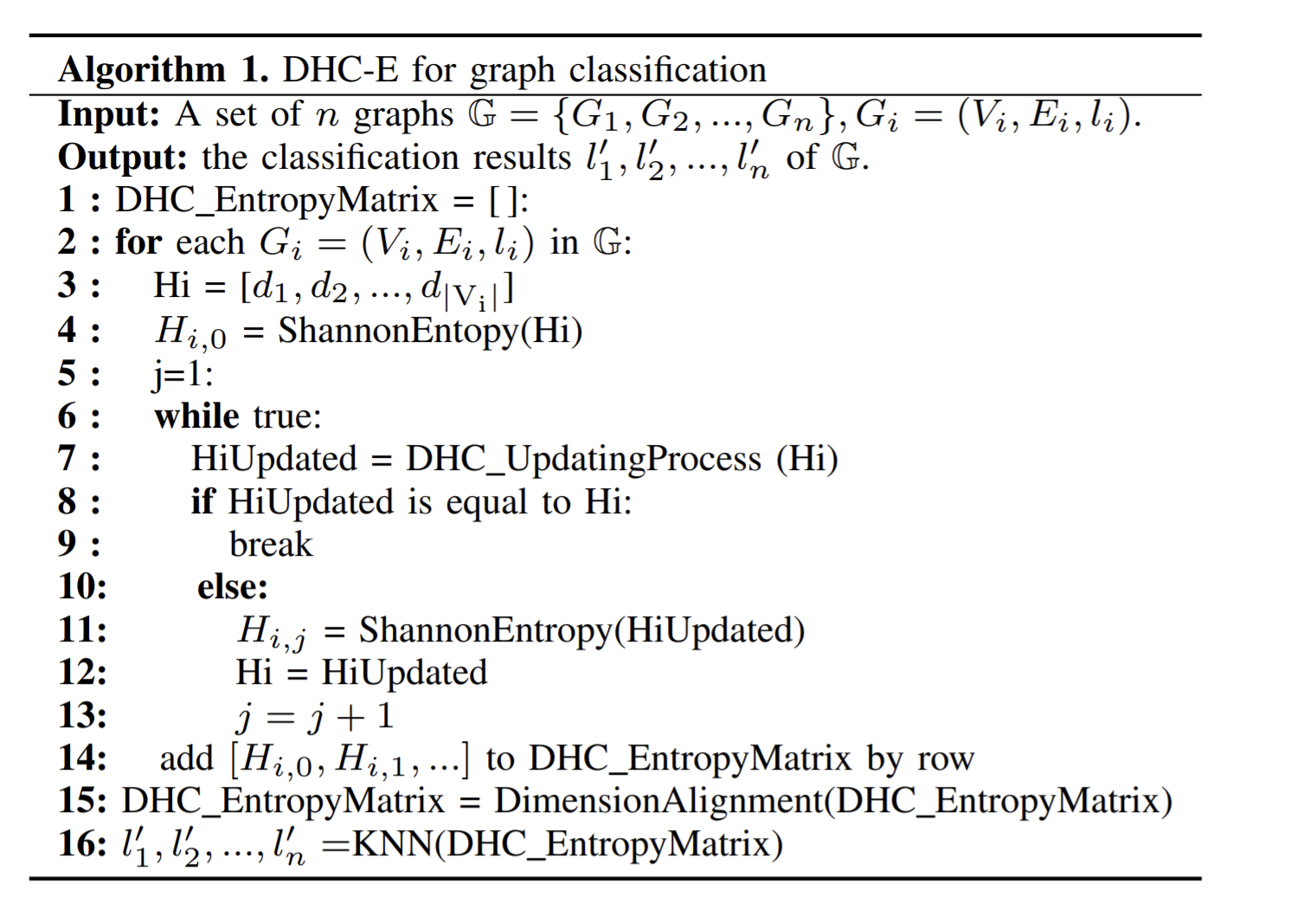
Paper 22: Infograph: Unsupervised and semi-supervised graph-level representation learning via mutual information maximization

Codes: https://github.com/fanyun-sun/InfoGraph

Why

• Traditional graph kernel based methods are simple, yet effective for obtaining fixed-length representations for graphs but they suffer from poor generalization due to hand-crafted designs
• one of the most difficult obstacles for supervised learning on graphs is that it is often very costly or even impossible to collect annotated labels.
• the handcrafted features of graph kernels lead to high dimensional, sparse or non-smooth representations and thus result in poor generalization performance, especially on large datasets.
• Deep Graph InfoMax (DGI) aims to train a node encoder that maximizes mutual information between node representations and the pooled global graph representation.
• Mean Teacher adds a loss term which encourages the distance between the original network’s output and the teacher’s output to be small. The teacher’s predictions are made using an exponential moving average of parameters from previous training steps.
• Explicitly extracting the graph can be more straightforward and optimal for graph-oriented tasks

Goal

• Graph-level representations learning
• maximize the mutual information between the graph-level representation and the representations of substructures of different scales
• Propose InfoGraph and InfoGraph* for unsupervised and semi-supervised separately. The InfoGraph* employs a student-teacher framework similar to Mean-Teacher method. It deploys two separate encoders but instead of explicitly encouraging the output of the student model to be similar to the teacher model’s output, they enable the student model to learn from the teacher model by maximizing mutual information between intermediate representations learned by two models.

How

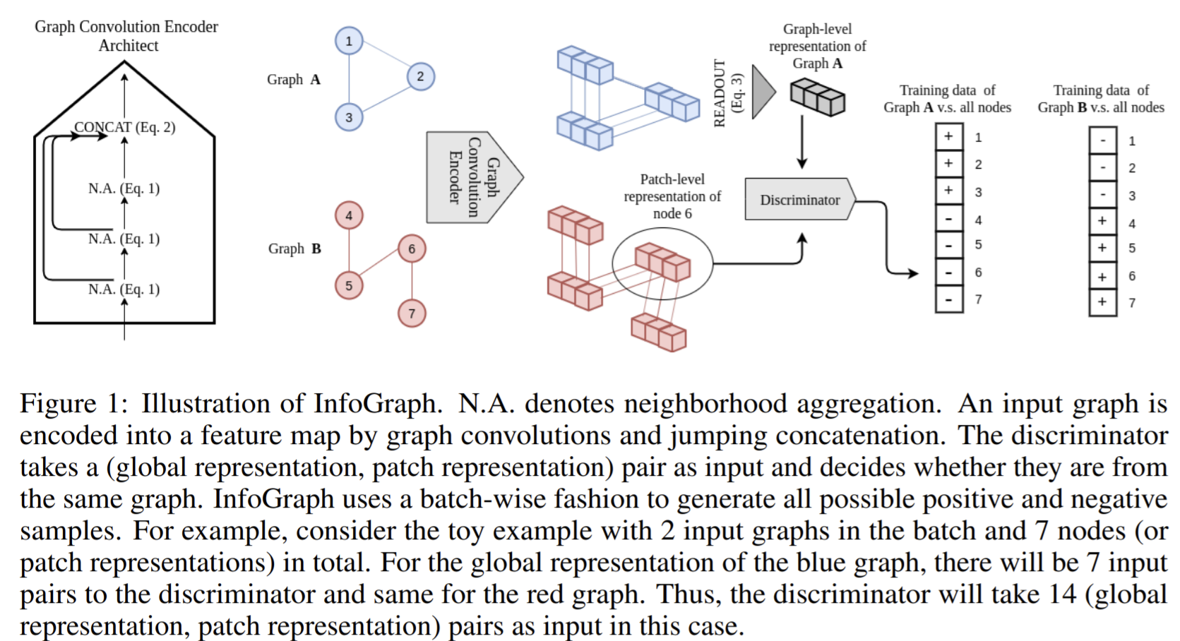
InfoGraph

• The encoder is GNN, finally the representations from different GNN layers are concatenated and readout (they use sum over mean ) as the global representations.
• The MI is between global and local pairs, and is estimated by Jensen-Shannon MI estimator.
• In practice, the negative samples are generated using all possible combinations of global and local patch representations across all graph instances in a batch.
• Although similar to DGI, they show their difference in
  1. They extract global representations rather than node-level representations
  2. For graph convolution encoders, they use GIN rather than GCN since GIN provides a better inductive bias for graph level representations.

InfoGraph*

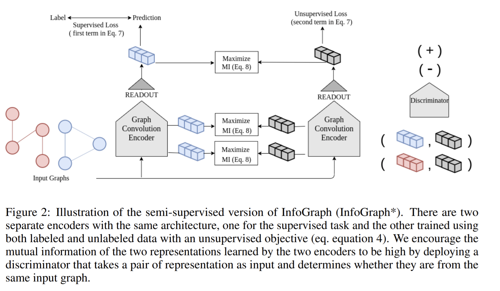
• Simply combining the two loss functions using the same encoder may lead to “negative transfer" (transfer knowledge from a less related source and thus may hurt the target performance).

• Therefore, they propose a simple way to alleviate this problem: deploy two encoder models: the encoder on the labeled data and the encoder on the unlabeled data. For transferring, they define a loss term that encourages the representations learned by the two encoders to have high mutual information, at all levels of representations.

  

• The formulation can be seen as a special instance of the student-teacher framework.

• To reduce computation cost, instead of enforcing the mutual-information maximization over all the layers of the encoders, at each training update, they enforce mutual-information maximization on a randomly chosen layer of the encoder.

Paper 23: Iterative graph self-distillation

Why

• The limitation of existing GNN architecture is that they often require a huge amount of labeled data to be competitive but annotating graphs.==> unsupervised learning such as graph kernels and matrix factorization.
• SSL
  • pretext task: needs meticulous designs of hand-crafted tasks
  • contrastive learning via InfoMax principle:
    • context-instance contrastive approaches usually need to sample subgraphs as local views to contrast with global graphs. And they usually require an additional discriminator for scoring local-global pairs and negative samples, which is computationally prohibitive. The performance is also very sensitive to the choice of encoders and MI estimators
    • context-instance contrastive approaches cannot be handily extended to the semi-supervised setting since local subgraphs lack labels that can be utilized for training.
• In order to alleviate the dependency on negative samples mining and still be able to learn discriminative graph representations, they propose to use self-distillation as a strong regularization to guide the graph representation learning.
• GCC (graph contrastive coding ): leverage instance discrimination as the pretext task for structural information pre-training.
• GraphCL: learn generalizable, transferrable, and robust representations of graph data in an unsupervised manner. Focuses on the impact of various combination of graph augmentation on multiple datasets and studies unsupervised
• Self-distillation is a special case when two architectures are identical, which can iteratively modify regularization and reduce over-fitting if perform suitable rounds.
• Semi-supervised learning
  • multi-task learning: regularizing the learning process with unlabeled data
  • consistency training between two separate networks: student-teacher framework, : introducing a slow-moving average teacher network to measures consistency against a student one, thus providing a consistency-based training paradigm where two networks can be mutually improved
• Data augmentation: limited since defining views of graphs is a non-trivial task.
  • Feature-space augmentation
  • structure-space augmentation

Goal

• Learn graph-level representations unsupervised by iteratively performing the teacher-student distillation with graph augmentations.
• Propose IGSD (iterative graph self-distillation), which constructs the teacher with an exponential moving average of the student model and distills the knowledge of itself.
• Extend IGSD to semi-supervised by jointly regularizing the network with both supervised and unsupervised contrastive loss.
• Seeking an approach that learns the entire graph representation by contrasting the whole graph directly alleviates the need for MI estimation, discriminator and subgraph sampling.

How

• Intuition: predict the teacher network representation of the graph pairs under different augmented views.
• Define a similarity metric for consistency-based training. The parameters of the teacher network are iteratively updated as an exponential moving average of the student network parameters.
• To extend to semi-supervised learning, they develop a self-training algorithm based on the supervised contrastive loss for fine-tuning.
• To perform augmentation, they have two choices
  • Transform a graph with transition matrix via graph diffusion and sparsification into a new graph with adjacency matrix as an augmented view in their framework
  • Randomly remove edges of graphs to attain corrupted graphs as augmented views.

Iterative graph self-distillation framework

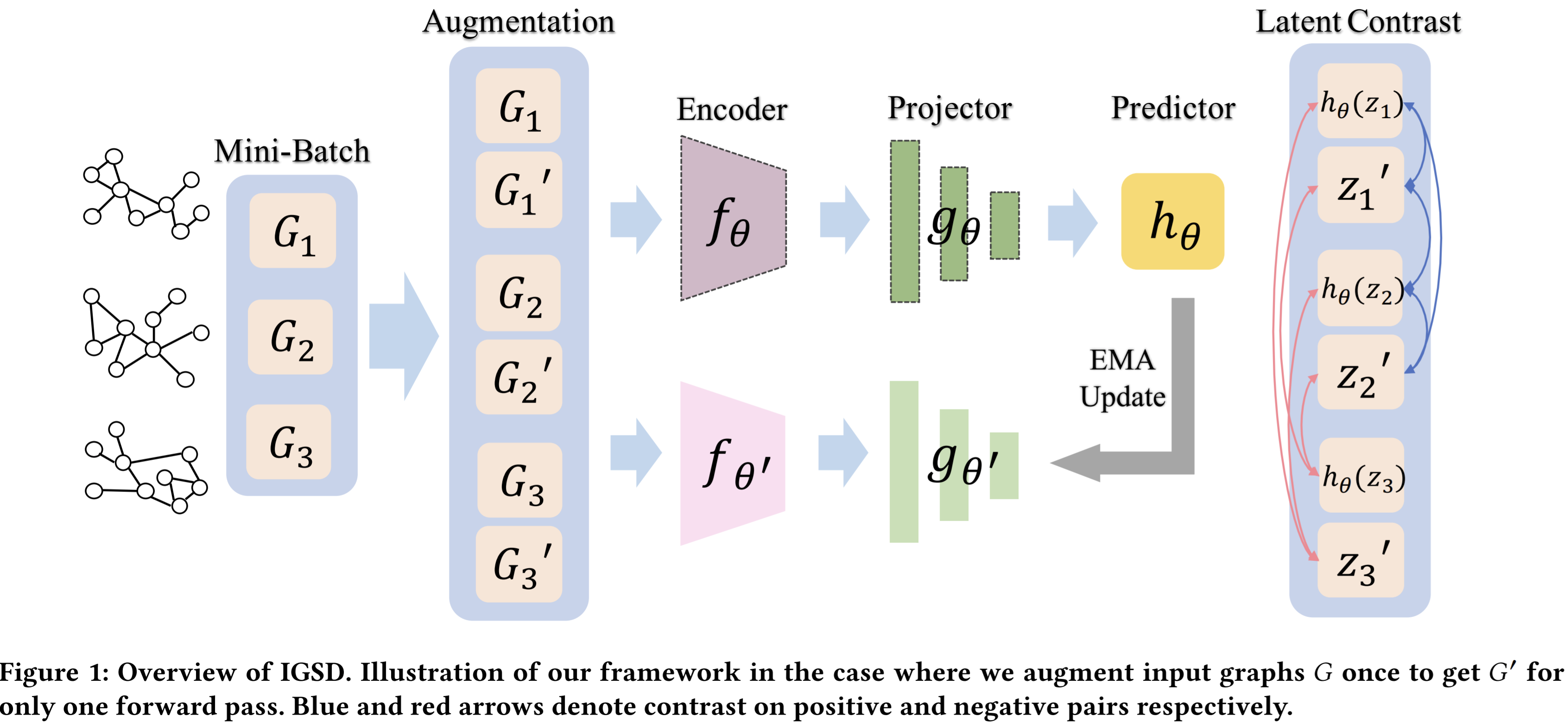
• Introduce a teacher-student architecture comprises two networks in similar structure composed by encoder \(f_\theta\), projector \(g_\theta\) and predictor \(h_\theta\). Denote the components of the teacher network and the student network as \(f_{\theta'},g_{\theta'}\) and \(f_{\theta},g_{\theta},h_\theta\) respectively.
• The positive pairs: the original and augmented view of the same graph, they are input into two networks respectively.
• The teacher's parameters are updated as an exponential moving average of the student parameters \(\theta\) after weights of the student network have been updated using gradient descent.
• The moving average network to produce prediction targets, enforcing the consistency of teacher and student for training the student network.

Self-supervised learning with IGSD

• Employ the Self-supervised InfoNCE objective.
• Obtain the graph representation by interpolating the latent representations with Mixup function.

Semi-supervised learning with IGSD

• The instance-wise supervision limited to standard supervised learning may lead to biased negative sampling problems.
• enforce consistency constraints between latents from different views, which acts as a regularizer for learning directly from labels
• train the model using a small amount of labeled data and then fine-tune it by iterating between assigning pseudo-labels to unlabeled examples and training models using the augmented dataset.

Paper 24: Learning by Aligning Videos in Time

Why

• To learn perfect alignment of two videos, a learning algorithm must be able to disentangle phases of the activity in time while simultaneously associating visually similar frames in the two different videos.
• Using temporal alignment for learning video representations
  • some use cycle-consistency losses to perform local alignment between individual frames.
  • some have explored global alignment for video classification and segmentation.
• Supervised methods require fine-grained annotations which can be prohibitively expensive.
• DTW is a global alignment metric, taking into account entire sequences while aligning, but not differential. The soft-DTW is differential.
• Video-based SSL representation learning
  • predict future frames or forecast their encoding features
  • leverage temporal information such as temporal order and temporal coherence.
• TCC (temporal cycle consistency ): learns Self-supervised representations by finding frame correspondences across videos.
  • But TCC aligns each frame separately, not like this paper which aligns the video as a whole.

Goal

• SSL for learning video representations using temporal video alignment as a pretext task.

How

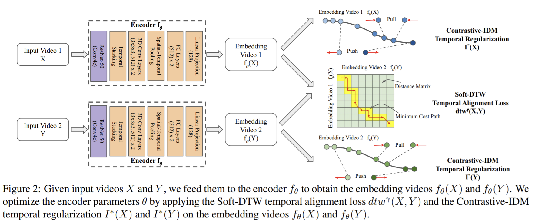
• Soft-DTW for the minimum cost for temporally aligning videos in the embedding space. And to avoid trivial solutions, they propose a temporal regularization term which encourages different frames to be mapped to different points in the embedding space
• Denote the embedding function as \(f_\theta\). They methods takes as input two videos \(X,Y\) with \(n,m\) frames respectively.

Temporal alignment loss

• For two videos \(X,Y\), after obtaining their embedding videos, one can compute the distance matrix \(D\). DTW calculates the alignment loss by finding the minimum cost path in \(D\): \(dtw(X,Y)=\min_{A\in A_{n,m}}\langle A,D \rangle\), where \(A_{n,m}\subset \{0，1\}^{n\times m}\) is the set of all possible alignment matrices, which correspond to paths from the top-left corner of \(D\) to the bottom-right Corner of \(D\) using only \(\downarrow,\rightarrow, \searrow\) moves.
  • \(A(i,j)=1\) if \(x_i\) in \(X\) is aligned with \(y_i\) in \(Y\).
  • This can be computed by dynamic programming.
• Because the \(\min\) operator, the DYW is not differentiable, to change it, soft-DTW is proposed
  • Replace the \(\min\) by the smoothed \(\min^\gamma\) one, defined as \(\min^{\gamma}\{a_1,a_2,\cdots,a_n\}=-\gamma\log\sum\limits_{i=1}^{n}e^{-\frac{-a_i}{\gamma}}\).
  • It returns the alignment cost between \(X,Y\) by finding the soft-minimum cost path in \(D\).
  • The smoothed \(\min^{\gamma}\) operator converges to the discrete \(\min\) when \(\gamma\) approaches 0.
  • \(\min^\gamma\) help the optimization by enabling smooth gradients and providing better optimization landscapes.

Temporal regularization

• To avoid trivial solutions (\(X,Y\) are mapped to a small cluster in the embedding space), they add a temporal regularization, which is separately applied on \(f_\theta(X),f_\theta(Y)\).

• Adapt inverse difference moment (IDM) as their regularization, which is written as:

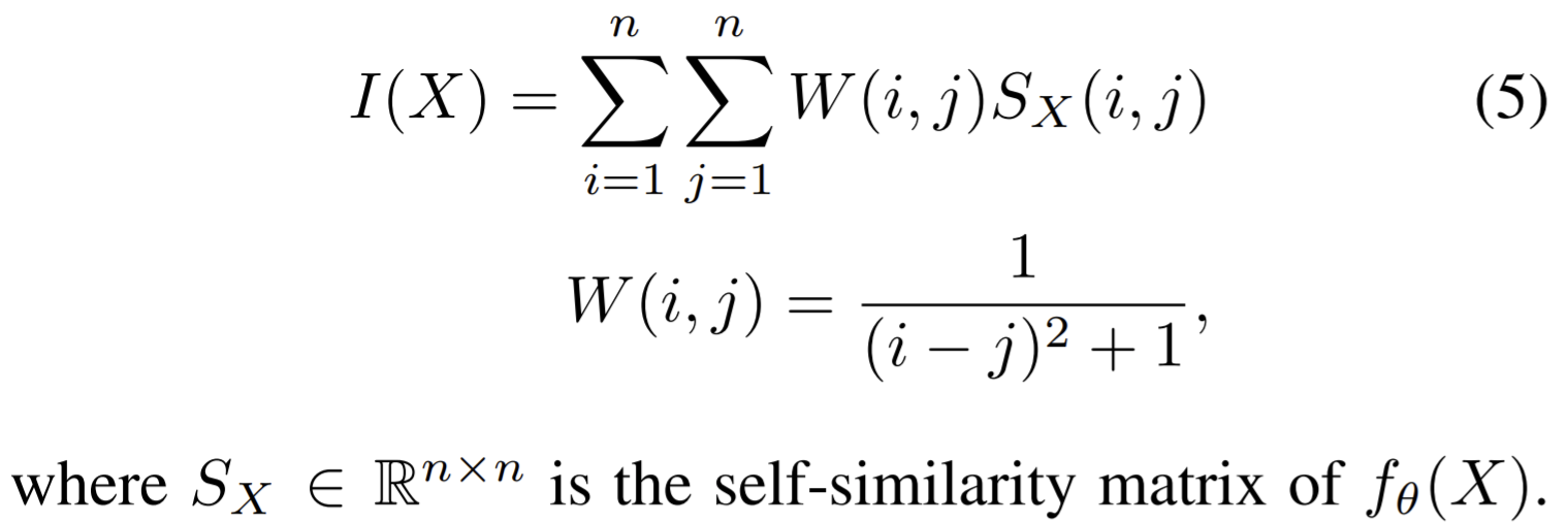
  • maximizes this equation encourages temporally close frames in \(X\) to be mapped to nearby points in the embedding space.

• But the equation above treats temporally close and far away frames in similar ways

  • They propose separate terms for temporally close and far away frames.

  • Introduce a contrastive version and named as contrastive-IDM.

    

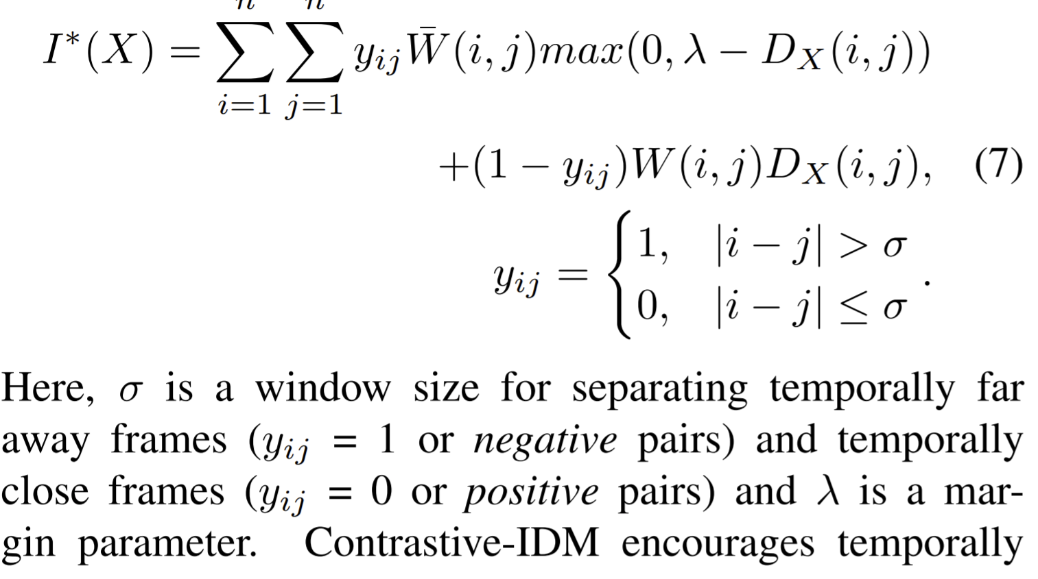
  • It encourages temporally close frames (positive pairs) to be nearby in the embedding space, while penalizing temporally far away frames (negative pairs) when the distance between them is smaller than margin \(\lambda\) in the embedding space.

  • Leveraging temporal information by adding weights to different pairs based on their temporal gaps leads to performance gain.

Final loss

• Combine soft-DTW alignments loss and contrastive-IDM:
• It encourages embedding videos to have minimum alignment costs while encouraging discrepancies among embedding frames.

Encoder network

• Use resnet-50 as backbone, stack \(k\) context frame features along the temporal dimension for each frame.
• Then the combined features are passed through two 3DCNN layers for aggregating temporal information.

Paper 25: Learning graph representation by aggregating subgraphs via mutual information maximization

Why

• Labeling graphs procedurally using strong prior knowledge is costly.
• Previous work
  • Graph kernel methods
    • Decompose the graph into several subgraphs and then measure similarities between them
    • much work on deciding the most suitable sub-structures by hand-craft similarity measures between sub-structures.
  • Semi-supervised learning
    • pseudo label methods: regard the prediction of unlabeled data as a pseudo label of unlabeled data, then train the network with all data together, and use a low weight of the loss of the unlabeled data part
    • Laddar network: combined supervised learning with unsupervised learning in DNNs to apply unlabeled data information to supervised learning reasonably.
  • learning by mutual information
    • express the amount of information shared between two random variables
    • But to alleviate computational cost, many approximation methods for mutual information are proposed.

Goal

• SSL to enhance graph-level representations with a set of subgraphs
• Separate the aggregation into three aspects and they design three information aggregators: attribute-conv, layer-conv, subgraph-conv. The attribute-conv aggregate the original information from graphs, the layer-conv aggregate the multi-hop node representations from different GNN layers. The subgraph-conv aggregate the information from the generated subgraphs.

How

• To constraint, maximizes the mutual information between the reconstructed graph representations rather than between graph and node representations as in previous works.
• a head-tail contrastive construction to provide abundant negative samples.
• In subgraph-agg stage, they introduce an auto-regressive method which is a universal SSL framework for the graph generation.

Node-agg stage

• Perform the MLP and AGG+MLP on node attributes and edge attributes firstly.
• The kernel size is \((2,1)\), which can squeeze each perspective of embeddings to one channel.

Layer-agg stage

• After perform convolution on the initial node representations for \(L\) layers, to aggregate the node representations of different scales so that local and global information can be combined organically, they propose to use a \((L,1)\) convolution kernel, named as layer-conv.
• Then the whole graph representations are obtained by a readout function.

Subgraph-agg stage

• Propose subgraph-agg, like an ensemble learning, since the nodes and graph representations do not express the same level of information
• Maximizing the mutual information between nodes and graph representation is not good enough to achieve the purpose of graph representations to express more information
• Steps
  • Build an autoregressive model to generate subgraphs from the original graph first
  • Assemble these subgraphs into a reconstructed graph \(\mathrm{G}^{rec}\). Use layer-conv, by maximizing the mutual information between two graphs representations in the same level, the graph representation is learned.
    • This mutual contrastive leads to lower variance than node-graph constrain.
• Auto-regressive subgraph generation
  • 
• Graph reconstruction
  • The readout function is used to aggregate each subgraph's representation.
  • Since there are \(S\) subgraphs, the kernel size of subgraph-conv is \((S,1)\), and the resulting representation is taken as the representation of the reconstructed graph \(\mathrm{G^{rec}}\)

Implementation

• By softmax, the output matrix \(P\) divides the original graph into two subgraphs, since \(p_{ij}\) denotes the probability that the node \(i\) is in the subgraph \(j\).
• To implement the auto-regressive paradigm of subgraph generation, there are two approaches
  • Tree-split generation
    • recursively utilize the basic operator to the newly generated subgraph. Just lie splitting a binary tree.
    • At each non-leaf node, they execute the softmax to partition graphs.
    • After \(T\) rounds split, they will get \(2^T\) subraphs.
  • multi-head generation
    • Import \(S\) learnable matrices to execute the softmax and get \(S\) partition matrices.
    • In this way, \(S\) subgraphs are selected in parallel but they break the rule of auto-regressive generation.
    • By assuming all subgraphs are conditionally independent concerning the original graph, one can take this method as an auto-regressive way.
• Loss function
  • The mutual information estimator is Jensen-Shannon divergence
  • The positive samples are the output of subgraph-conv.
  • Ways to get easy negative samples
    • using different graphs in the batch
    • or use the corruption function to get negative samples from the original graph.
  • For a graph, its hard negative pair sample can be built by shuffling the node embeddings.
• 

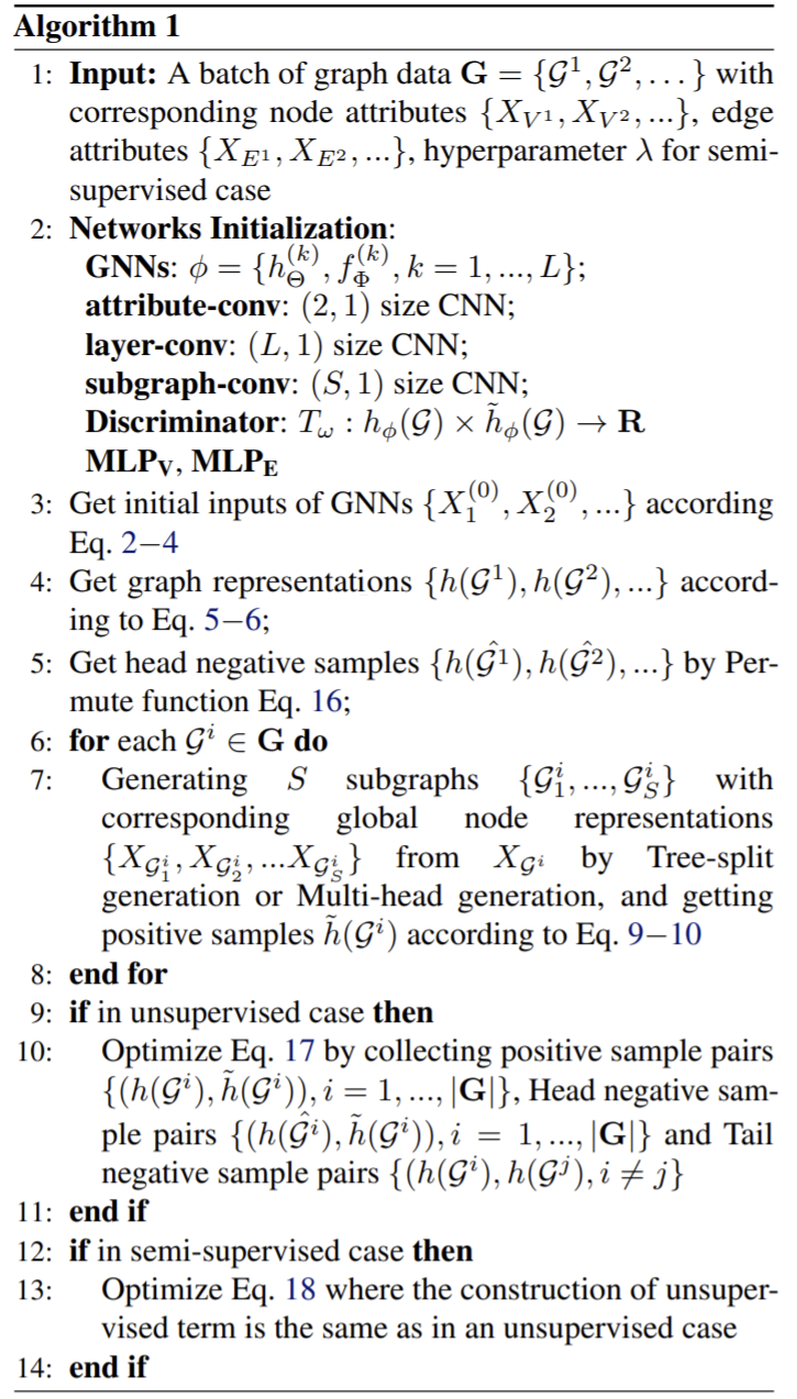
Paper 26: Mile: A multi-level framework for scalable graph embedding

Codes: https://github.com/jiongqian/MILE

Why

• None of the existing efforts examines how to scale up graph embedding in a generic way.
• HARP is familiar with this work: but it focuses on improving the quality of embeddings by using the learned embeddings from the previous level as the initialized embeddings for the next level. But the way it is extended to other graph embedding is not obvious.
• the quality of such embedding methods be strengthened by incorporating the holistic view of the graph.

Goal

• Obtain graph embedding efficiently and effectively (save computation cost), introduce MILE (multi-level embedding framework), allow contemporary graph embedding methods to scale to large graphs.
• Given a graph \(\mathcal{G} = (V, E)\) and a graph embedding method \(f(\cdot)\), we aim to realize a strengthened graph embedding method \(\hat{f}(\cdot)\) so that it is more scalable than \(f(\cdot)\) while generating embeddings of comparable or even better quality.

How

• repeatedly coarsen the graph into smaller ones by employing a hybrid matching strategy
• compute the embeddings on the coarsest graph using an existing embedding technique
• propose a novel refinement model based on learning a graph convolution network to refine the embedding from the coarsest graph to the original graph.

Graph coarsening

• the set of nodes forming a super-node is called a matching
• Structural Equivalence Matching (SEM): Given two vertices \(u,v\) in an unweighted graph \(\mathcal{G}\), we call they are structurally equivalent if they are incident on the same set of neighborhoods. Since if two vertices are structurally equivalent, then their node embeddings will be similar.
• Normalized Heavy Edge Matching (NHEM): select an unmatched node, say \(u\), in the graph and find a large weighted edge \((u, v)\) incident on node \(u\) such that node \(v\) is also unmatched. Then collapse nodes \(u,v\) into one super-node and mark them as matched. The edge weights are normalized. The normalized method penalizes the weights of edges connected with high-degree nodes.
• Define matching matrix to store the matching information from graph \(\mathcal{G}_i\) to \(\mathcal{G}_{i+1}\) as a binary matrix, the \(r\)-the row and \(c\)-the column of \(M_{i,i+1}\) is set to 1 if node \(r\) in \(\mathcal{G}_i\) collapse to super-node \(c\) in \(\mathcal{G}_{i+1}\), and is set to 0 if otherwise.
• vertices with a small number of neighbors have a limited choice of finding a match and should be given a higher priority for matching. Otherwise, once their neighbors are matched by others, these vertices cannot be matched.
• The embeddings learned by base embedding method on the coarsened graph can act as an effective initialization for the graph-topology aware refinement model.
• Choice of coarsening level: depends on the application domain and the graph properties

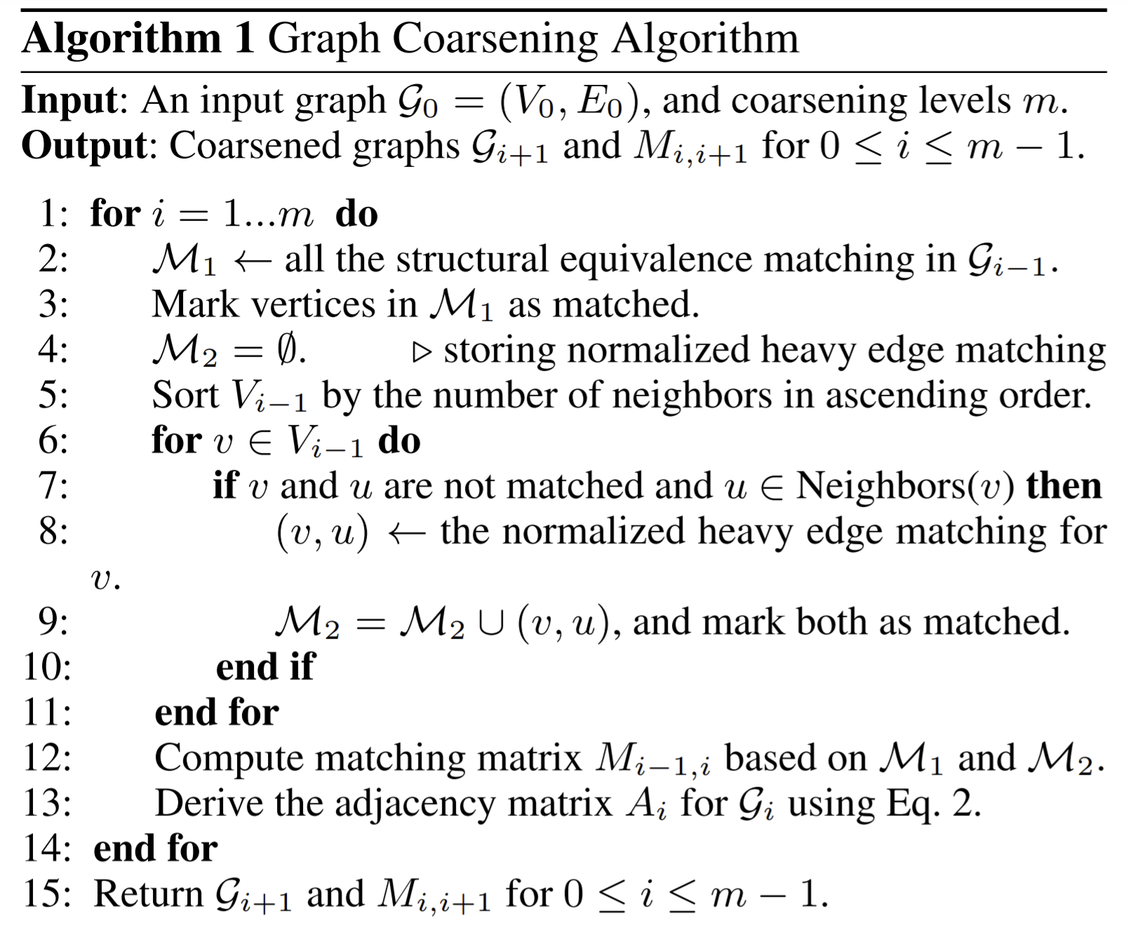
Base embedding on coarsened graph

• They can use any graph embedding algorithm for base embedding.

Refinement of embeddings

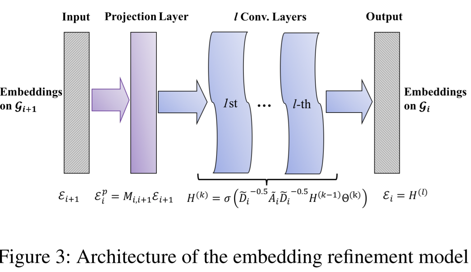
• Given the series of coarsened graph and their corresponding matching matrix, and the node embeddings on \(\mathcal{G}_m\), they seek to develop an approach to derive the node embeddings of \(\mathcal{G}_0\) from \(\mathcal{G}_m\).

• Subtask:

  • Propose to use GCN. Since the simple project will induce \(\mathcal{E}_i^p\) from \(\mathcal{E}_{i+1}\), but one limitation is that nodes will share the same embeddings if they are matched and collapsed into a super-node during the coarsening phase.
  • The GCN uses the projected embedding \(\mathcal{E}_i^p\) and the adjacency matrix \(A_i\) from the input graph. Define the embedding refinement model as a \(l\)-layer graph convolution model:
  • The intuition behind this refinement model is to integrate the structural information of the current graph \(\mathcal{G}_i\) into the projected embedding \(\mathcal{E}_i^p\) by repeatedly performing the spectral graph convolution.

• Choice of number of GCN layers: \(l\) GCN layers correspond to aggregating structural information from all the \(l\)-hop neighbours for each node.

  • But large \(l\) will make the node embeddings homogeneous and less distinguishable across the graph due to the small-world property of real-world graphs.
  • In practice, they use 2.

• Train refinement model

  • learn \(\Theta^{(k)}\) on the coarsest graph and reuse them across all the levels for refinement

  • The loss function is defined as the MSE, where the ground truth is a base embedding on \(\mathcal{G}_i\).

    • But two drawbacks: The above loss function requires one more level of coarsening to construct \(\mathcal{G}_{m+1}\) and an extra base embedding on \(\mathcal{G}_{m+1}\). Also, the embedding space of graph \(\mathcal{G}_{m}\) and \(\mathcal{G}_{m+1}\) can be totally different since the two embeddings are learned independently.
    • One possible solution for these drawbacks may be force the embeddings to be aligned between the two graphs.

  • Finally, this paper propose to construct a dummy coarsened graph by simply copying \(\mathcal{G}_m\), i.e. \(M_{m,m+1}=I, \mathcal{G}_{m+1}=\mathcal{G}_m\).

    • reduce one iteration of graph coarsening
    • avoid performing base embeddings on \(\mathcal{G}_{m+1}\).

    

    • Adopt gradient-descent with BP to learn parameters.

• 

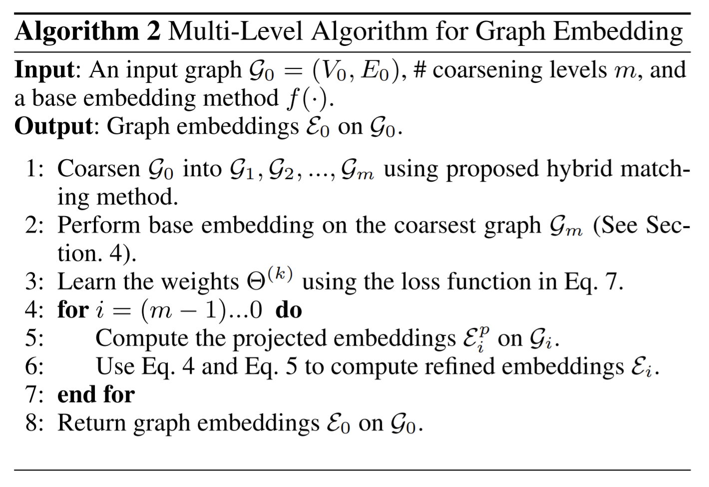
• The shared \(\Theta^{(k)}\) values do much better than alternative \(\Theta^{(k)}\).

Paper 27: Missing Data Estimation in Temporal Multilayer Position-aware Graph Neural Network (TMP-GNN)

Not clear for me.

Why

• The goal of node embedding methods: identify a vector representation that captures node location within a broader topological structure of the graph. But most focus on static graphs.
• To deal with dynamic graphs
  • One way is to use a GNN based node embedding for each individual time layer and aggregate the results accordingly.==> ignore inter-layer correlation.
  • P-GNN: learn position-aware node embedding that utilize local network structure and the global network position of a given node with respect to randomly selected nodes called anchor-sets that enables us to distinguish among isomorphic nodes.

Goal

• Propose TMP-GNN (Temporal multi-layered positio-aware GNN), a node embedding method for dynamic graphs. (change over time: edges, nodes attributes etc.)
• The method in this paper is an extension of static position-aware GNN (P-GNN).

How

• exploit a supra-adjacency matrix to encode a temporal graph with its intra-layer and inter-layer coupling in a single graph.
• use hidden states learned from bi-directional GRU (bi-GRU) to learn the long-term temporal dependencies in both forward and backward directions to estimate missing values.
• conditional centrality derived from eigenvector based centrality to distinguish nodes of higher influence

Notations and preliminaries

• The existence of inter-layer edge is restricted between separate instances of same nodes from one layer to another. The inter0later edge weight between two layers is identical for all nodes in those layers.
• To model the coupling between two layers, this paper couples the adjacent time layers by neglecting the directionality of time, considering the short term dependencies between time layers.
• Supracentrality matrix
  • A temporal graph is represented through a sequence of adjacency matrices that each of which refers to one layer of a dynamic network at a specific point of time.
  • The supracentrality matrix \(\mathbb{C}(\omega)\) is built by linking up centrality matrices across time layers through a weighted inter-layer parameter \(\omega\) (used to adjust the extent of coupling strength among pair of time layers.)
    • When \(\omega\rightarrow\infin\), the centrality measures change slowly over time, \(CC_{v}(\omega)\) reaches to stationary that is equal to average \(CC_{v}(\omega)\) over all time layers.
    • On the other hand, small \(\omega\) makes \(CC_{v}(\omega)\) fluctuate fromega one time layer to the other.
  • Each item of \(\mathbb{C}(\omega)\) shows joint centrality, the importance of every node-layer pair \((v,t)\). Additionally marginal and conditional centralities are defined to represent the relative importance of a node compared to other nodes at time layer \(t\).
  • \(\mathbb{C}(\omega)\) consists of \(\hat{\mathbb{C}}=diag [\mathrm{C^{(1)},\cdots,C^{(T)}}]\) and \(\omega\hat{\mathbb{A}}\), where \(\hat{\mathbb{C}}\) represents a set of \(T\) weighted centrality matrix of individual layers, and the latter encoder the uniform and diagonal coupling with strength parameter \(\omega\) between the time layers. Only consider the coupling among same nodes between consecutive pair of layers.
• To solve, the dominant eigenvector \(\mathbb{V}(\omega)\) is corresponds to largest eigenvalues \(\lambda_{max}\), . The elements in \(\mathbb{V}(\omega)\) are interpreted as scores that measure the importance of node-layer pairs \((v,t)\).
• Conditional centrality of node \(v\), denoted as \(CC_{v}(\omega)\), shows the importance of the node relative to other nodes at layer \(t\).

TMP-GNN

• Position-aware GNN rather than original one, which aggregates the positional and feature information of each node with randomly selected number of nodes called anchor-sets.
• The goal is to find the best position-aware embedding \(\mathrm{z}_v^t\) with minimum distortion for a given node \(v\) at time layer \(t\).
• Modifications to P-GNN:
  • Generalization of P-GNN to time varying graphs: Adopt the input of P-GNN as supracentrality matrix, the embedding \(\mathrm{z}_v^t\) will then be aggregated from an RNN based representation to estimate missing data.
  • modification of \(\mathcal{M}_j\): Using attention while calculating a message from anchor-set containing node \(u\) with respect to a given node \(v\). Attention is used to learn the relative weights between the feature vector of \(v\) and its neighbor \(u\) from the anchor-set.
    • The \(\mathcal{M}_j\) for anchor-set, denoted as \(M_v[j]\), is obtained by the shortest path between a pair of nodes and mean of \(\mathcal{M}_j\).
  • Modification of \(AGG_{\mathcal{R}}\): \(\mathcal{R}\) denotes the anchor-set. Corresponding informative anchor-sets contain at least 1-hop neighbours of node \(v\). Of those neighbor nodes, the ones with higher \(CC_v(\omega)\) deserve to have higher \(r_j\) for aggregation.
    • Large anchor-sets have higher probability of hitting \(v\), but are less informative of positional information of the node, as \(v\) hits at least one of many nodes in the anchor-sets.
    • Small anchor-sets have fewer chance of hitting \(v\), but provide positional information with high certainty.
• Edge embedding is estimated by averaging the embedding of the ending nodes.

Bi-directional RNN

• Take \(Z_e,M_e,\Delta_e\) as input, where \(Z_e\) is randomly masked by removing missing points and set it to zero. The \(\Delta_e\) illustrates the time difference between the current and the last layer which the measurement is recorded. It's defined to handle the different sampling rate associated with data heterogeneity from different sources.
• Goal: Find the best estimate \(\mathrm{\hat{x}_{e_d}^t}\) with minimum RMSE for a particular missing point.
• Versions
  • The E-TMP-GNN I aims at extracting additional features out of the embedding yields from TMP-GNN, and use it to further enrich the edge feature sets.
  • TMP-GNN II aims at reducing the number of feature streams by implementing a softmax layer.

Paper 28: Multi-Level Graph Contrastive Learning

Why

• Most graph representation learning methods using GNN focus on supervised fashion and heavily depend on label information.

• Unsupervised methods

  • many reconstruction-based unsupervised algorithms have been proposed, either reconstruct the features of graph nodes or the topology structure of the graph.

• SSL methods

  • contrastive methods, propose many data augmentation methods

    

    

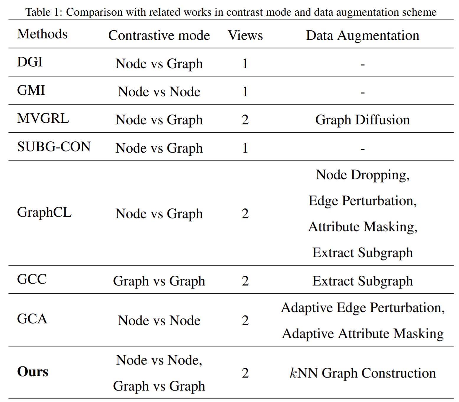
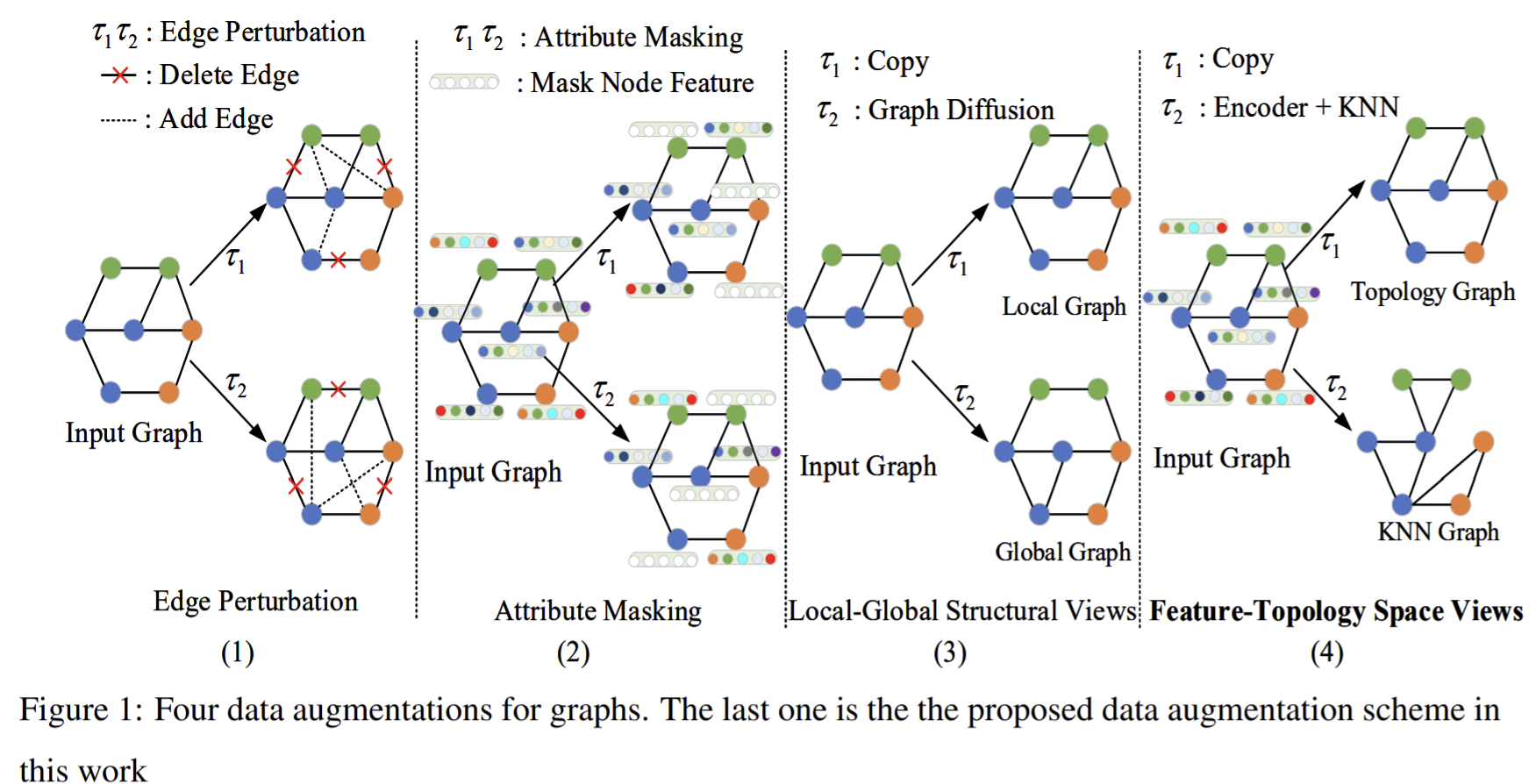
    • shuffles node features to augment the training examples
    • multi-view, maximizes MI between node representations of one view and graph representation of another view
    • subgraphs: MI loss defined on central nodes and their sampled subgraphs representation.
    • GCA: adaptive augmentation, extract the important connective structures of the original graph to the augmentation data based on node centrality measures.
    • GraphCL: multiple augmentation, including edge perturbation, attribute masking, and maximizes the MI between the node and global semantic representations to learn node representations.

• GNN does not perform well on disassortative graphs. Constructing a KNN graph by feature similarity or dropping the links between nodes indifferent classes are feasible methods.

• Contrastive learning consists of three main components: data augmentation schemes, the learner model and loss function

  • data augmentation: design according to the priors and properties of graph-structured data:
    • vertex and edge missing do not alter the graph semantics;
    • the missing partial attributes of each node does not alter the robustness of the graph semantics;
    • the subgraph structure of the graph can hint full semantics;
    • correlated views of the same graph possess semantic consistency.
  • Loss function
    • Probability loss: Deepwalk, node2vec. Maximizes the probability of nearest vertices of the given vertex to learn graph representation. Nodes occurring in the same sequence are viewed as the positive samples, and they should have similar representation.
    • Adversarial loss: generative-contrastive
    • Triplet loss: an important role in deep metric learning. Given an anchor \(x\), a positive \(x_p\) of the same class as the anchor, a negative \(x_f\) of a different class, the triple loss targets at achieving that the distance of \(x,x_f\) greater than the distance of \(x,x_p\) plus margin \(m\). \(\max(d(x,x_p)-d(x,x_f)+m)\).
    • Contrastive loss: maximizing the similarity of the corresponding nodes between two views, or maximizes the MI between node and graph representation.

Goal

• SSL for graph node representation learning
• propose a Multi-Level Graph Contrastive Learning (MLGCL) framework for learning robust representation of graph data by contrasting space views of graphs. Introduce a contrastive view-topological and feature space views. Adopt KNN graph (generated by encoding features preserves high-order proximity).
• Feature space+topology space. The correlated graphs have similar and intrinsic characteristics.
• Contrastive learning aims to learn an encoder model \(f(\cdot)\) which can learn a robust representation for each node \(v_i\) that is insensitive to the perturbation caused by data augmentations \(\tau\).

How

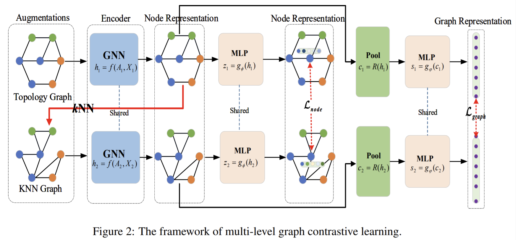
• First sample a pair of graph augmentation functions \(\tau_1,\tau_2\) from augmentation pool \(\tau\), which is applied to the input graph to generate the augmented graph of two views. Then use a pair of the shared GNN-based encoder to extract node representation, and further employ the pooling layer to extract the graph representation. Then use the shared MLP layer to project the nodes representations from both views into the space where the node-level contrastive loss is computed. \(\tau_2\) includes an encoder and KNN function.

Data augmentation

• exert perturbation on the input graph to generate two correlated graphs of the same graph. Extract augmentation graph structure from space view.
• Given the graph structure of topology space \(G(A,X)\) , extraction is done
  • First employ GNN encoder to extract the encoding features \(Z\) of topology graph
  • Then apply kNN to \(Z\) to construct KNN graph with community structure \(G_f(A_f,X)\), where \(A_f\) is the adjacency matrix of KNN graph.
    • First calculate the similarity matrix \(S\) based on \(N\) encoding features \(Z\). The choice of similarity function can be Mahalanobis distance, cosine similar or gaussian kernel. They use cosine similarity in their experiments.
    • Then choose top \(k\) similar node pairs for each node to set edges and finally get the adjacency matrix of KNN graph \(A_f\).

GNN Encoder

• Learn node representation \(z_1,z_2\) for two augmented graphs. In inference phase, only use GNN encoder to learn node representation for downstream tasks.
• Given topology graph \(G(A,X)\), KNN graph \(G_f(A_f,X)\), employ a two-layer GCN as the encoder.
• For node representation \(Z_a,Z_b\) of each view, use a graph pooling layer to derive their graph representation.

MLP and graph pooling

• MLP: maps the representation to the space in which the contrastive loss is computed. Since two views, there are two MLP.
• Graph pooling: readout layer, used to learn graph representation.

Multi-level loss function

• Used to preserve the low-level "local" and high-level "global" agreement, simultaneously.
• Consists of two parts: the contrast of low-level node representation between two views, and the contrast of high-level graph representation between two views.
• Positive samples \((z_i^a,z_i^b)\), K-1 pair of negative samples \((z_i^a,z_j^a),(z_i^a,z_j^b)\).

Paper 29: Permutation-Invariant Variational Autoencoder for Graph-Level Representation Learning

Why

• unsupervised learning on graphs mainly focus on node-level representation learning, which aims at embedding the local graph structure into latent node representations.
  • Usually implemented by an autoencoder framework
• A graph-level representation should not depend on the order of the nodes in the input representation of a graph.

Goal

• Graph-level unsupervised learning
• Propose a permutation-invariant variational autoencoder for graph structured data. The method indirectly learns to match the node ordering of input and output graph, without imposing a particular node ordering or performing expensive graph matching

How

• Address the order ambiguity issue by training alongside the encoder and decoder model an additional permuter model that assigns to each input graph a permutation matrix that aligns the input graph node ordering with the output graph ordering.

Problem definition

• Consider a dataset of graphs \(\mathrm{G}={\mathcal{G}^{(i)}}_{i=0}^N\), the goal is to represent in a low-dimensional continuous space. Assume the data is generated by a process \(p_\theta(\mathcal{G}|\mathrm{z})\), then approximate the intractable posterior by \(q_\phi(\mathcal{G}|\mathrm{z})\) and minimize the lower bound on the marginal likelihood of graph \(G^{(i)}\):
  • The KL-divergence divergence term regularizes the encoded latent codes of graphs \(\mathcal{G}^{(i)}\)
  • The second term enforce high similarity of decoded graphs to their encoded counterparts
  • Parameters \(q_\phi,p_\theta\) can be estimated by NNs that encode and decode node features \(\mathrm{X}_\pi^{(i)}\) and adjacency matrices of graphs \(\mathcal{G}^{(i)}\).
• Considering the permutation invariant, \(\mathcal{G}_\pi,\hat{\mathcal{G}}_{\pi'}\) have to be brought in the same node ordering.
• Previous work either fail to track \(\mathrm{P}_{\pi'\rightarrow \pi}\), or is computational costly (by maximizing the similarity which involves up to \(O(n^4)\) re-ordering operations at each training step).

Permutation-Invariant variational graph autoencoder

• Propose to silver the reordering problem implicitly by inferring the permutation matrix \(\mathrm{P}_{\pi'\rightarrow\pi}\) from the input graph \(\mathcal{G}_\pi\) by a model \(g_\psi(\mathrm{P}|\mathcal{G}_\pi)\).

• Train this model jointly with the encoder model \(q_\phi(\mathrm{z}|\mathcal{G})\) and decoder model \(p_\theta(\mathcal{G}|\mathrm{z})\).

  

• The permuter model has to learn how the ordering of nodes in the graph generated by the encoding model will differ from a specific node ordering present in the input graph. It predicts for each node \(i\) of the input graph a score \(s_i\) corresponding to its probability to have a lower node index in the decoded graph.

• Next they derive the elements of the permutation matrix \(\mathrm{P}\) by sorting the scored nodes: \(p_{ij}=\begin{cases}1,& ifj=\arg sort(s)_i\\0,&else\end{cases}\). The argsort is then replaced by the continuous relaxation: ， where the softmax operator is applied row-wise, \(d(x,y)\) is the \(L_1\)-norm and \(\tau\) a temperature-parameter.

• The permuter model \(g_\psi\) is trained with stochastic gradient descent.

• In order to push the relaxed permutation matrix towards a real permutation matrix (only one 1 in every row and column), add a row- and column-wise entropy term as additional penalty term to equation (5)

  

• By enforcing \(C(\mathrm{P})=0\), the real permutation matrix is fulfilled.

Details of the model architecture

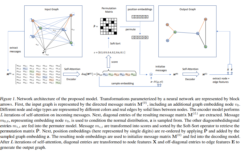
• Graph representation by directional messages: MPNN
  • Key idea: aggregation of neighborhood information by passing and receiving messages of each node to and from neighbouring noes in a graph. In \(k\) hop.
  • The item \(m_{ij}\) of message matrix \(\mathrm{M}\) is \(m_{ij}=\sigma([x_i\|x_j\|e_{ij}]\mathrm{W+b})\).
  • Nodes in this view are represented by self-message \(\mathrm{diag(M)}\).
• Self-attention on directed messages
  • Embedded in MPNN, take the message matrix to compute key,value and query.
  • Let messages \(m_{ij}\) only attend on incoming messages \(m_{ki}\) to reduce the complexity.
• Encoder
  • A dummy node \(v_0\) acts as an embedding node, the cumulated messages are updated in \(m_{0,0}\).
  • Then use the reparameterization trick and sample the latent representation \(\mathrm{z}\) of a graph by sampling from a multivariate normal distribution.
• Permuter
  • to predict how to re-order the nodes in the output graph to match the ordering of nodes in the input graph.
  • After extract node embeddings represented by self messages on the main diagonal of the encoded message matrix, retrieve the permutation matrix \(\hat{\mathrm{P}}\) by scoring these messages with a function which is parameterized by a linear layer and the soft-sort operator.
• Decoder
  • Add position embeddings to the initial node embeddings, same as what's defined in Bert. And then the permutation matrix is performed on these position embeddings. After obtaining the permutation matrix, extracted messages are permuted by the permutation matrix and then use self-attention in decoder to extract node and edge features.
  • Pad all graphs in a batch with empty nodes to match the number of nodes of the largest graph, attention on empty nodes is masked out at all time.

Paper 30: PiNet: Attention Pooling for Graph Classification

Codes: http://github.com/meltzerpete/pinet

Why

• The essential to the success of CNNs is the process of pooling
  • Pooling is invariance to different orderings of the input vectors.
  • GCNs achieve invariance by pooling neighbors' feature vectors with symmetric operators such as feature-weighted mean, max, and self-attention weighted means.
• Previous work on permutation invariant
  • Propose a permutation invariant function \(f(\mathbb{X})\) on the set \(\mathbb{X}\) may be learned indirectly through decomposition in the form \(f(\mathbb{X})=\rho(\sum\limits_{x\in\mathrm{X}}\phi(x))\). The model is named as Janossy pooling, where \(\rho\) is a normalization function, and the summation occurs over the set of all possible permutations of the input set.
  • The use of canonical orderings to tackle permutations in graph representation learning has been demonstrated to be effective in Patchy-SAN.
  • DGCNN uses a sorting method to introduce permutation invariance.
  • Variants may also be expressed as an instance of the WL graph isomorphism algorithm.
• A simple solution is to use a symmetric operator to combine vertex vectors to form a single graph vector.

Goal

• graph classification
• A generalized differential attention-based pooling mechanism for utilizing graph convolution operations for graph-level classification.
• The proposed pooling mechanism is differentiable, by which the vertex-level invariance to permutation achieved for vertex level tasks may be extended to the graph level.

How

• 
• The inner softmax constrains the attention coefficients to sum to 1 and prevents them from all falling to 0. The outer softmax may be replaced for multi-label classification tasks (i.e. sigmoid).

Paper 31: Self-supervised Graph-level Representation Learning with Local and Global Structure

Codes: https://github.com/DeepGraphLearning/GraphLoG

Why

• Existing methods mainly focus on preserving the local similarity structure between different graph instances but fail to discover the global semantic structure of the entire dataset.
• a desirable graph representation should be able to preserve the local-instance structure. It should also reflect the global-semantic structure of the data.
• Require a model that is sufficient to model both the local and global structure of a set of graphs

Goal

• Study the unsupervised/self supervised graph-level representation
• propose a unified framework called Local-instance and Global-semantic Learning (GraphLoG) for self-supervised whole-graph representation learning
• Introduce hierarchical prototypes to capture the global semantic clusters.
• EM for training

How

• To preserve local similarity between various graph instances, align the embeddings of correlated graphs/subgraphs by discriminating the correlated graph/subgraph pairs from the negative pairs.
• Import hierarchical prototypes to depict the latent distribution of a graph dataset in a hierarchical way. Propose to maximizes the data likelihood with respect to both the GNN parameters and hierarchical prototypes via an online EM algorithm.
  • E-step, infer the embeddings of the mini-batch of graphs sampled from the data distribution with a GNN, and sample the latent variable of each graph from the posterior distribution defined by current model.
  • M-step, maximizes the expectation of complete-data likelihood with respect to the current model by optimizing with a mini-batch-induced objective function.

Problem definition

• Expect the graph embeddings \(\mathrm{H}=\{h_{\mathcal{G}_1},\cdots,h_{\mathcal{G}_M}\}\) follow both the local-instance and global-semantic structure.
  • Local-instance structure: For a pair of similar graphs/subgraphs, \(\mathcal{G,G'}\), their embeddings are expected to be nearby in the latent space.
  • Global-semantic structure: After mapping to the latent space, the embeddings of a set of graphs are expected to form some global structures reflecting the clustering patterns of the original data.
• Since \(h_v\) summarizes the information of a subgraph centered around node \(v\), they refer \(h_v\) as subgraph embedding. Then the entire graph's embedding is derived as \(h_\mathcal{G}=f_{\mathcal{R}}(\{h_v|v\in\mathcal{V}\})\), where \(f_{\mathcal{R}}\) is a permutation-invariant readout function, like mean pooling.
• EM
  • In E-step, using the observed \(\mathrm{X}\) and pre-estimated \(\theta_{t-1}\) to estimate the posterior \(p(\mathrm{Z|X,}\theta_{t-1})\)
  • In M-step, use the posterior to calculate the expectation of \(\log p(\mathrm{X,Z|}\theta)\), and \(\theta_t\) is the solution of maximizing this expectation.

GraphLoG

• Learning local-instance structure of graph representation

  • The problem is formulated as maximizing the similarity of correlated graph/subgraph pairs while minimizing that of negative pair.
  • Given a graph sampled from the data distribution, obtain its correlated counterpart through randomly masking a part of node/edge attributes in the graph.
    • Given a molecular graph, we randomly mask the attributes of 30% nodes (i.e. atoms) in it to obtain its correlated counterpart. Specifically, we add an extra dimension to the feature of atom type and atom chirality to indicate masked attribute, and the input features of all masked atoms are set to these extra dimension.
  • The similarity function is cosine similarity.
  • The negative pairs: for a correlated graph pair \(\mathcal{G,G'}\) or correlated subgraph pair \(\mathcal{G_v,G'_v}\), substitute \(\mathcal{G(G}_v)\) randomly with another graph from the dataset (a subgraph centered around another node in the same graph) to construct negative pairs.
  • The local-instance structure of graph representations is then solved by minimizing \(\mathcal{L}_{graph}+\mathcal{L}_{sub}\).

• Leaning global-semantic structure of graph representation

  • Hierarchical prototypes to represent the feature clusters in the latent space in a hierarchical way. Each layer has several prototypes.

  • encourage the graphs to be compactly embedded around corresponding prototypes and, at the same time, refine hierarchical prototypes to better represent the data. Formalize the problem as optimizing a latent variable model.

  • To solve parameters: hierarchical prototypes \(\mathrm{C}\), the online EM is applied.

    • The online EM is base on i.i.d. assumption, where both the complete-data likelihood and the posterior probability of latent variables can be factorized over each observed-latent variable pair

      

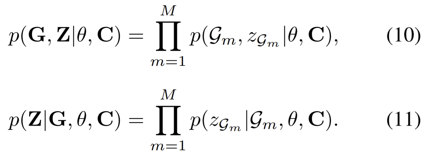
    • The initialization of model parameters

      Pretrained GNN by minimizing \(\mathcal{L}_{local}\) and employ the derived GNN model as initialization, then use it to extract the embeddings of all graphs in the data set. After, k-means clustering is applied upon these graph embeddings to initialize the bottom layer prototypes with the output cluster centers.

      The prototypes of upper layers are initialized by iteratively applying kmeans to the prototypes of the layer below.

      Clusters with less than two samples are dropped.

    • E-step

      • randomly sample a mini-batch of graphs. Each latent variable is a chain of prototypes from top layer that best represent graph \(\mathcal{G}_n\) in the latent space.
      • To train, use stochastic EM algorithm, draw a sample for Monte Carlo estimation.
      • Formally, we first sample a prototype from top layer according to a categorical distribution over all the top layer prototypes. For the sampling at layer \(l\) (\(l > 2\)), we draw a prototype from that layer based on a categorical distribution over the child nodes of prototype sampled from the layer above.

    • M-step: Maximizes the expected log-likelihood on mini-batch to obtain \(\theta,\mathrm{C}\).

  • This algorithm can indeed maximizes the marginal likelihood function \(p(\mathrm{G}|\theta,\mathrm{C})\).

• 

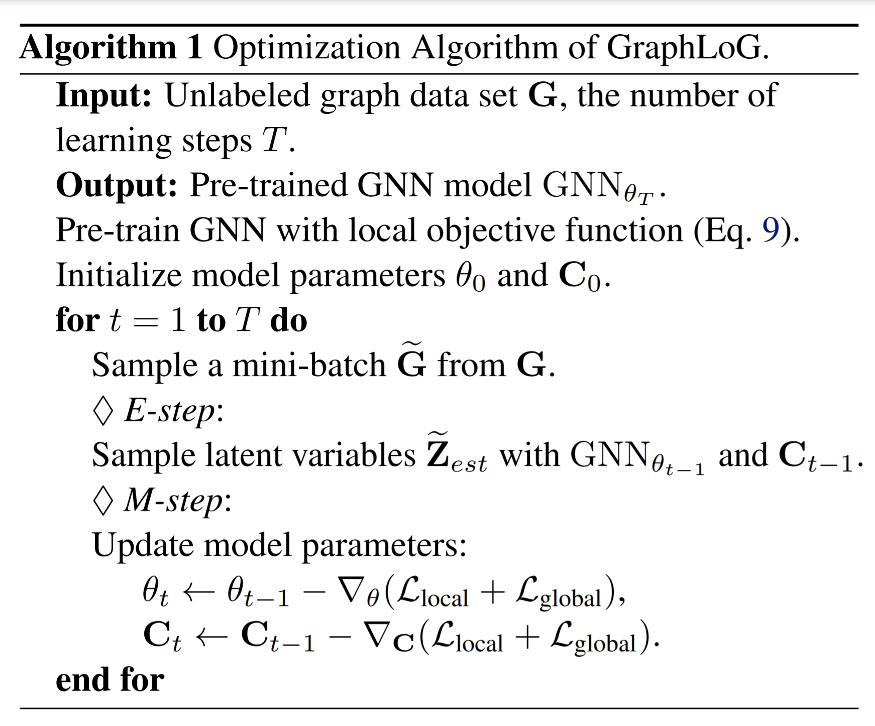
Paper 32: Self-supervised Heterogeneous Graph Neural Network with Co-contrastive Learning

Codes: https://github.com/liun-online/HeCo

Why

• HGNNs can effectively combine the mechanism of message passing with complex heterogeneity.
• Most methods on HGNN are semi-supervised, but the requirement of some node labels are known is not always fullfilled.
• Contrastive learning is able to learn the discriminative embeddings even without labels. But the following problems have to be addressed
  • How to design a heterogeneous contrastive mechanism
    • Different meta-paths (used to capture the long-rang structure in a HIN) represent different semantics.
    • Performing contrastive learning only on single meta-path view is actually is actually distant from sufficient.
  • How to select proper views in a HIN:
    • The selected view should cover both of the local and high-order structures while meta-path is usually used to extract the high-order structure. Meta-path is the combination of multiple relations, so it contains complex semantics, which is regarded as high-order structure.
    • Both of the network schema and meta-path structure views should be carefully considered.
  • How to set a difficult contrastive task
    • A proper contrastive task will further promote to learn a more discriminative embedding.
    • Need to make the contrastive learning on two not too similar views. One strategy is to enhance the information diversity in two views, the other is to generate harder negative samples of high quality.
• There is a lack of methods contrasting across views in HIN so that the high-level factors can be captured.

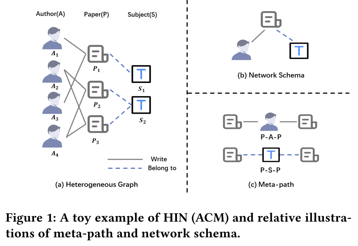
Goal

• Self-supervised on Heterogeneous graph neural networks (HGNNs), learn node embeddings.
• Propose a novel co-contrastive learning mechanism for HGNNs, named HeCo. It employs cross-view contrastive mechanism. Specifically , two views of a HIN, namely network schema and meta-path views are proposed to learn node embeddings.

How

• Choose network schema and meta-path structure as two views.
  • In network schema, the node embedding is learned by aggregating information from its direct neighbors.
  • In meta-path view, the node embedding is learned by passing messages along multiple meta-paths to capture high-order structure.
• To make contrast harder, propose a view mask mechanism that hides different parts of network schema and meta-path, respectively.
• Given the high correlation between nodes, define the positive samples of a node in HIN and design a optimization strategy specially.

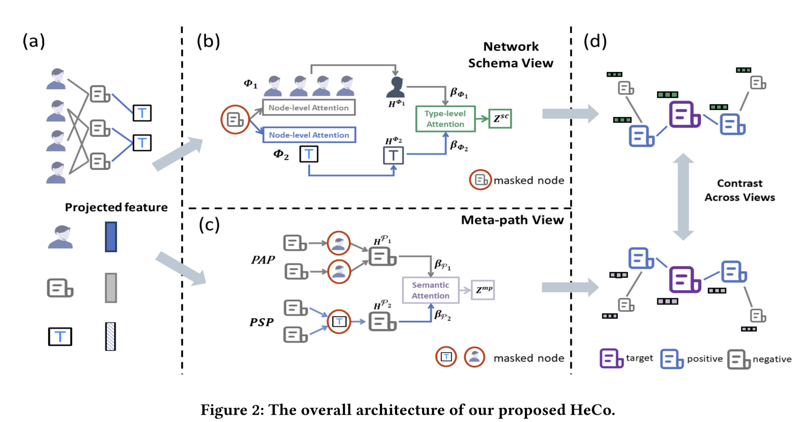
Node feature transformation

• First need to project features of all types of nodes into a common latent vector space to avoid features of nodes distributed into different spaces.
• For a node \(i\) with type \(\phi_i\), design a type-specific mapping matrix \(W_{\phi_i}\) to transform its feature \(x_i\) into common space as \(h_i=\sigma(W_{\phi_i}\cdot x_i+b_{\phi_i})\), where \(h_i\) is the projected feature of node.

Network schema view guided encoder

• Now aim to learn the embedding of node \(i\) under network schema view. For node \(i\), different types of neighbors contribute differently to its embedding, and so do the different nodes with the same type. Therefore, attention is used in node-level and type-level to hierarchically aggregate messages from other types of neighbors to target node \(i\).
• For node-level (same type) attention, the projected features of nodes \(h_i\) are used to calculate the attention map, then applied on projected features. Note that in practice, they randomly sample a part of neighbors (in the same type) for aggregation on one node. In this way, they ensure that every node aggregates the same amount of information from neighbors, and promote the diversity of embeddings in each epoch under this view.
• After getting all type embeddings, they use type-level attention to fuse them together to get the final embedding for node \(i\) under network-schema view. The attention here is apply tanh on linear combination of type embeddings.
  • Is \(\mathrm{a}_{sc}\) trainable here?

Meta-path view guided encoder

• Each meta-path represents one semantic similarity.
• For one meta-path \(\mathcal{P}_n\) from \(M\) meta-paths, apply meta-path specific GCN to encode, features will be \(h_j^{\mathcal{P}_n}=\frac{1}{d_i+1}h_i+\sum\limits_{j\in N_i^{\mathcal{P}_n}}\frac{1}{\sqrt{(d_i+1)(d_j+1)}}h_j\), where \(h_i,h_j\) are their projected features. For each node, along \(M\) meta-path, it will have \(M\) embeddings.
• Then to fuse \(M\) embeddings for each node, use semantic-level attention to get the final embedding under the meta-path view.
  • Is \(\mathrm{a}_{mp}\) trainable here?

View mask mechanism

• a view mask mechanism that hides different parts of network schema and meta-path views, respectively.

  

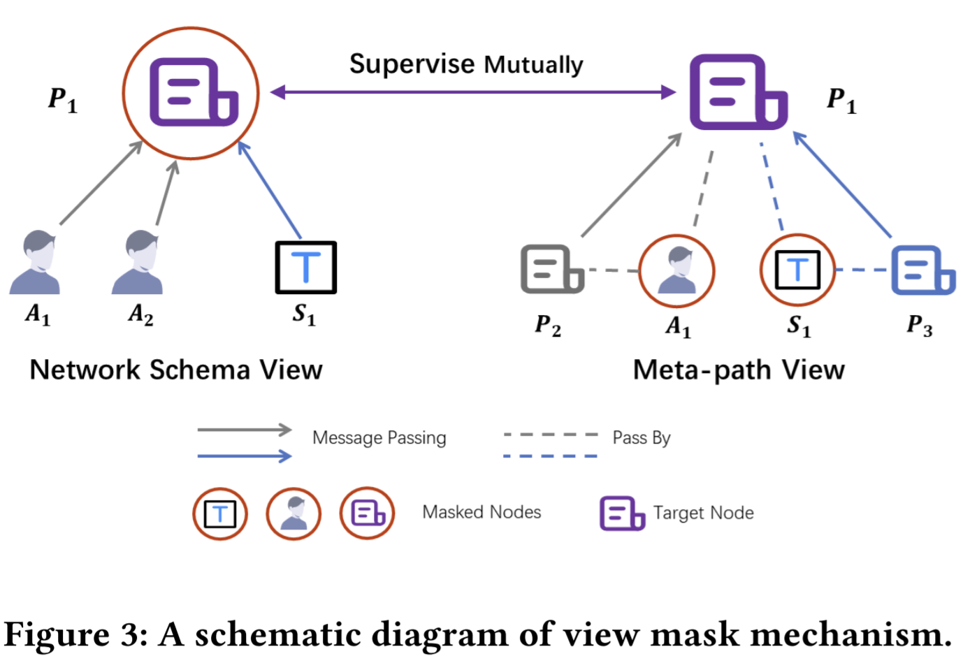
• How to select nodes? Still unclear for me.

Collaboratively contrastive optimization

• Feed the obtained features from two views to MLP to map them into the space where contrastive loss is calculated. Both views use the same MLP.
• Positive pairs and negative pairs
  • But consider that nodes are usually highly-correlated because of edges, propose a new positive selection strategy
    • if two nodes are connected by many meta-paths, they are positive samples. Then the selected positive samples can well reflect the local structure of the target node.
  • Steps
    • First count the number of meta-paths connecting two nodes
    • Then sort the node set \(S_i\) by this count in descending order and set a threshold \(T_{pos}\). If The count is larger than the threshold, select first \(T_{pos}\) nodes from \(S_i\) as positive samples of node \(i\).
    • Treat all left nodes as negative samples of \(i\).
  • Different from traditional methods, they consider multiple positive pairs.
  • In contrastive loss \(\mathcal{L}_i^{sc}\), for two nodes in a pair, the target embedding is from the network schema view and the embeddings of positive and negative samples are from the meta-path view. This also realize the cross-view self-supervision.
  • In contrastive loss \(\mathcal{L}_i^{mp}\), the target embedding is from the meta-path view while the embeddings of positive and negative samples are from the network schema view.
• The final loss is the combination of \(\mathcal{L}_i^{sc},\mathcal{L}_i^{mp}\), optimized by back propagation. The \(\mathcal{L}_i^{mp}\) is used to perform downstream tasks because nodes of target type explicitly participant into the generation of \(z^{mp}\).

Model extension

• HeCo_GAN
  • Sample additional negatives from a continuous Gaussian distribution.
  • Composed of three components: the proposed HeCo, a discriminatory D and a generator G.
    • Train D and G: first train D to identify the embedding from two views as positives and that generated from G as negatives. Then rain G to generate samples with high quality that fool D.
    • Use trained G to generate samples, which can be viewed as the new negative samples with high quality.
• HeCo_MU
  • Proposed to improve results in supervised learning by adding arbitrary two samples to create a new one.
  • Build hard negative samples: get cosine similarities between noes \(i\) and nodes from \(\mathbb{N}_i\) during calculating, and sort them in the descending order. Then select first top \(k\) negative samples as the hardest negatives, and randomly add them to create new \(k\) negatives, which are involved in training.
  • No learnable parameters in this version.

Paper 33: SM-SGE: A Self-Supervised Multi-Scale Skeleton Graph Encoding Framework for Person Re-Identification

Codes: https://github.com/Kali-Hac/SM-SGE

Why

• Previous works just learn body and motion features from the body-joint trajectory, whereas lack a systematic way to model body structure and underlying relations of body components beyond the scale of body joints.
  • extract appearance-based features such as body texture and silhouettes from RGB or depth images: but vulnerability to illumination or appearance changes
  • skeleton-based models: robust to factors such as view and body shape changes
• still an open challenge to extract discriminative body and motion features with 3D skeletons for person Re-ID
• Multi-scale skeleton graphs: many previous methods extract hand-crafted features from skeletons with a single spatial scale and topology
• Multi-scale relation learning: previous works mostly encode body-joint trajectory or pre-defined pose descriptors into a feature vector, rarely explore the inherent relations between different body joints or components.
• Multi-scale skeleton dynamics modeling: Previous methods mostly learn skeleton motion at a fixed scale of body joints, lack the flexibility to capture motion patterns at various levels==> cause a loss of global motion features.

Goal

• Person re-identification. Propose a Self-supervised Multi-scale Skeleton Graph Encoding (SM-SGE) framework that models human body, component relations, and skeleton dynamics from unlabeled skeleton graphs of various scales to learn an effective skeleton representation for person Re-ID.
• MGRN (multi-scale graph relation network) + MSR (multi-scale skeleton reconstruction), where MSR with two concurrent pretext tasks, namely skeleton subsequence reconstruction task and cross-scale skeleton inference task.
• No need of ID labels during training.
• Effective with the 3D skeletons estimated from RGB videos.

How

• First devise multi-scale skeleton graphs with coarse-to-fine human body partitions, which enables to model body structure and skeleton dynamics at multiple levels.
• To mine inherent correlations between body components in skeletal motion, propose a multi-scale graph relation network to learn structural relations between adjacent body-component nodes and collaborative relations among nodes of different scales.
• Propose a multi-scale skeleton reconstruction mechanism to enable to encode skeleton dynamics and high-level semantics from unlabeled skeleton graphs.
• The input is several clips of 3D skeleton sequence. First train to get representation \(\mathrm{H}\), then take the frozen \(\mathrm{H}\) and corresponding ID labels to train a MLP for person Re-ID.

MS skeleton graph construction

• Goal: learn a latent discriminative representation \(\mathrm{H}\) from skeleton sequences \(\mathrm{S}\) without using any label.

• regard body joints as the basic components, and merge spatially nearby groups of joints to be a higher level body-component node at the center of their positions. The graphs at joint-scale, part-scale and body-scale are denoted as \(\mathcal{G^1,G^2,G^3}\) respectively.

  

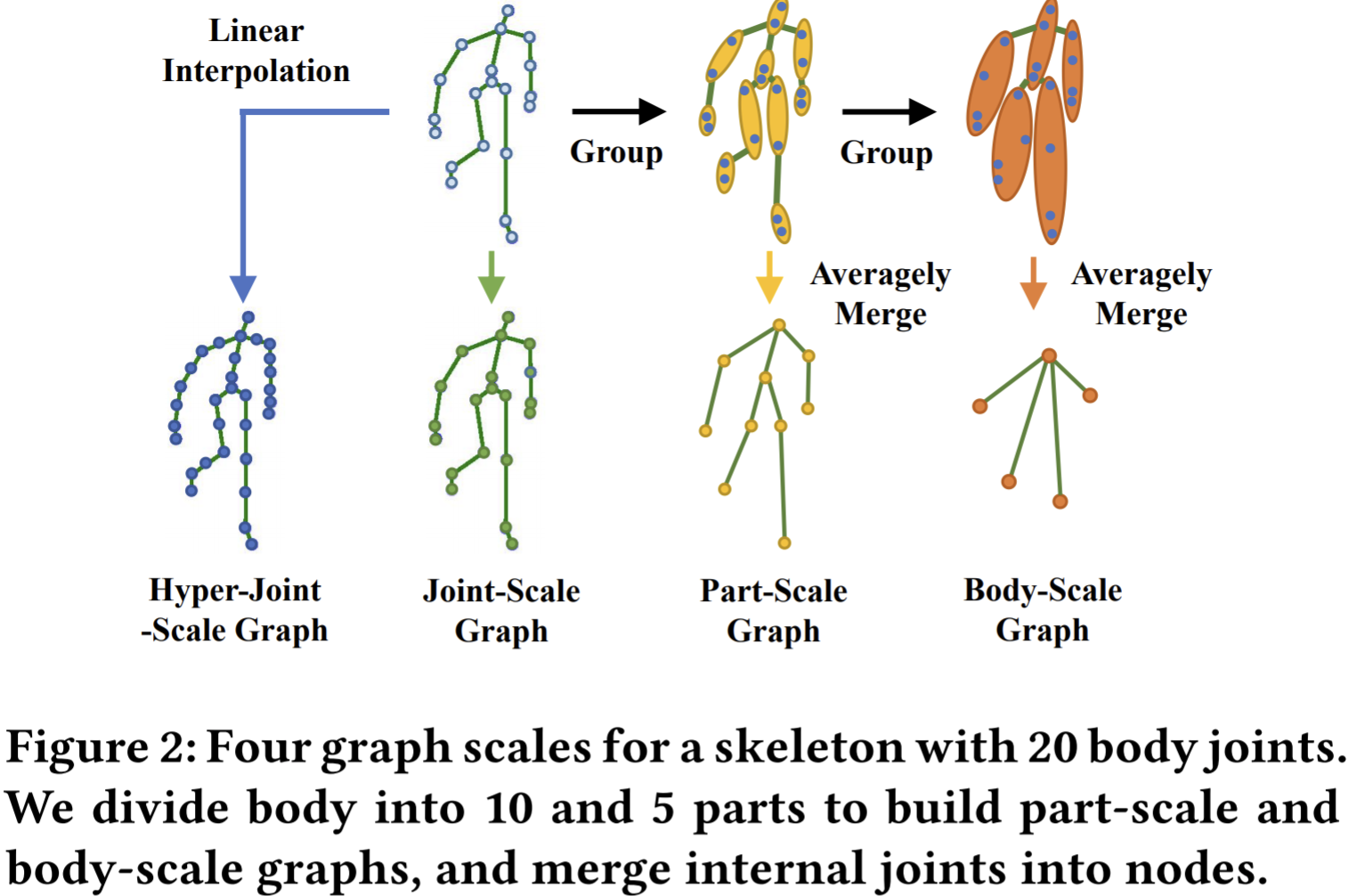
• The hyper-joint-scale is implemented by interpolating nodes between adjacent nodes.

MSGR

• Propose to learn relations of body components from two aspects: structural relations which provide a higher motion correlation than distant pairs, and collaborative relations that considers several action-related body components.

  

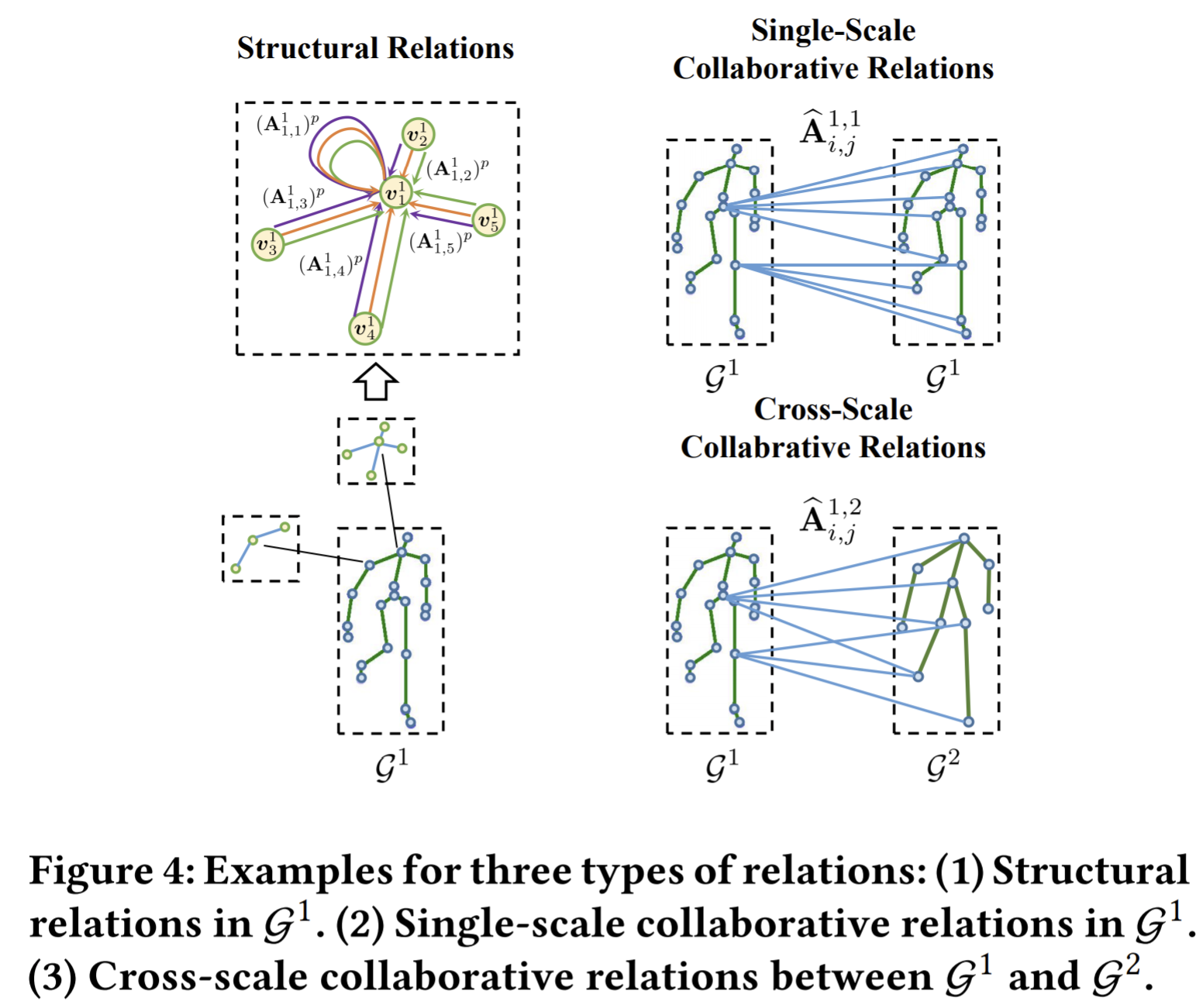
• Structural relation learning

  • First compute the structural relation between adjacent nodes as follows:
  • Then normalized relations with a temperature-based softmax (T-softmax) function to learn flexible structural relations. The higher value of temperature produces a softer relation distributed over nodes and retains more similar relation information.
  • The aggregate features of most relevant nodes to represent the node \(i\), in which both the \(v_j\) and the relation matrix \(\mathrm{A}_{i,j}^m\) are taken as the input.
  • The previous three steps are operated for \(P\) times to obtain \(P\) different structural relation matrices.
  • Then averagely aggregate features learned by these relation matrices to represent each node.

• Collaborative relation learning

  • Unique walking patterns could be represented by the dynamic cooperation among body joints or between different body components.
  • Learn collaborative relations from two aspects: single-scale collaborative relations among nodes of the same scale, and cross-scale collaborative relations between a node and its spatially corresponding or motion-related higher level body component.
  • Use softmax and the nodes features at different scale to obtain collaborative relation matrix, still the T-softmax. But calculate the inner product of node feature representations to measure the degree of collaboration between two nodes.

• Multi-scale collaboration fusion

  • Each node representation in the \(a\)-th scale graph is updated by the feature fusion of collaborative nodes from different graphs as where the \(\lambda_C\) is the fusion coefficient to fuse collaborative graph node features.
  • graph representations of each individual scale is retained to encourage their model to capture skeleton dynamics and pattern information at different levels

Multi-scale skeleton reconstruction mechanism

• Pretext tasks for capturing skeleton graph dynamics and high-level semantics from different scales of graphs.
• Skeleton subsequence reconstruction task: MSR aims to reconstruct target multi-scale skeletons corresponding to multi-scale graphs in subsequences, instead of reconstructing the original subsequences.
• Cross-scale subsequence reconstruction task: exploit fine skeleton graph representations to infer 3D positions of coarser body components. E..g., use joint-level graph representations to infer nodes of body-scale skeletons.
• To simultaneously achieve above two pretext tasks, first sample \(k\)-length subsequences by randomly discarding \((f-k)\) skeletons from the input sequence. The sampling process is repeated for \(r\) rounds and each round cover all possible lengths form 1 to \(f-1\).
  • Given a sampled skeleton subsequence, MGRN encodes its corresponding skeleton graphs of each scale into fused graph features as previously mentioned.
  • Then, leverage an LSTM to integrate the temporal dynamics of graphs at each scale into effective representations.
  • Last, use graph states at the \(𝑎^{𝑡ℎ}\) scale and MLP to reconstruct the target skeleton at the \(b^{𝑡ℎ}\) scale.
  • The reconstruction loss use \(\ell_1\) norm.

The entire framework

• For the downstream task, extract encoded graph states (𝒉) learned from the pre-trained framework, and exploit an MLP \((g(\cdot))\) to predict the sequence label .
• For the \(t^{th}\) skeleton in an input sequence, concatenate its corresponding encoded graph states of four scales as its skeleton-level representation of the sequence. Then train MLP with the frozen \(\mathrm{H}_t\) and its label. The predicted label is \((g(\mathrm{H}_t))\).

Paper 34: Space-time correspondence as a contrastive random walk

Codes: https://github.com/ajabri/videowalk

Why

• Challenge: temporal correspondence: a physical point depicted at position \((x,y)\) in frame \(t\) might not have any relation to what we find at that same \((x,y)\) in frame \(t+k\).
• Cycle-consistency of time is a promising direction.
  • current methods rely on complex and greedy tracking that may lead to local optima, especially when applied recurrently in time.

Goal

• self-supervised approach for learning a representation of visual correspondence from raw video, where correspondence means prediction of links in space-time graph constructed from video.
• Take patches sampled from each frame as nodes, and nodes adjacent in time sahre a directed edge. The long-range correspondence is computed as a walk along the graph.
• Optimize the representation to place high probability along paths of similarity.

How

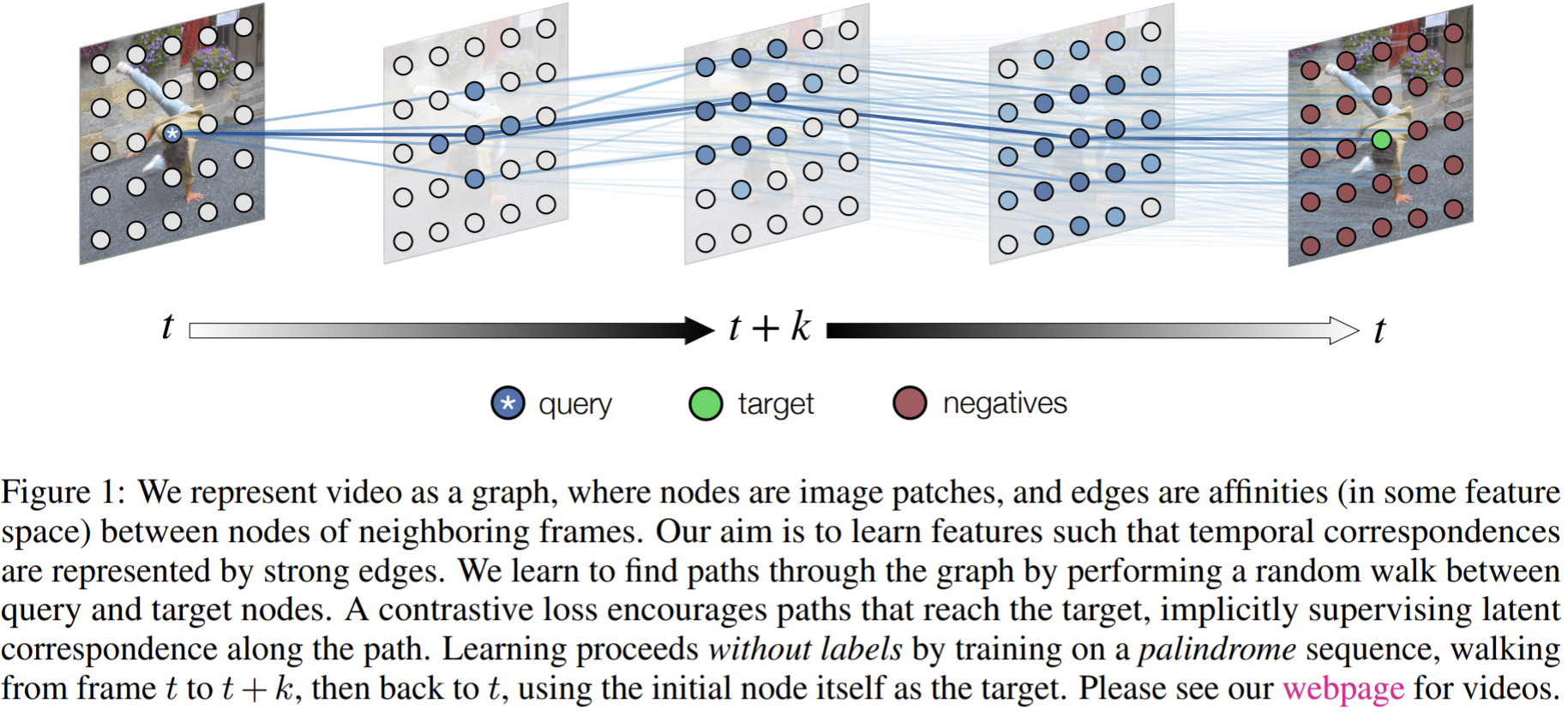
• Turn training videos into palindromes: sequences where the first half is repeated backwards. View each step of the walk as a contrasstive learning problem where the walker's target provides supervision for entire chains of intermediate comparisons.

Contrastive random walks on video

• An encoder \(\phi\) maps nodes to \(\ell_2\)-normalized \(d\)-dimensional vectors. The similarity function is non-neative affinities, the whole function of encoder is based on \(T\)-softmax, and the output is denoted as the stocastic matrix of affinities \(A_{t}^{t+1}\), which describes only the local affinity between the patches of two video frames \(\mathrm{q}_t,\mathrm{q}_{t+1}\). \(A_{t}^{t+1}\) is then used to build transition probabilities of a random walk on the whole graph, which relates all nodes in the video as a Markov chain.
  • The step of random Walker Can be viewed as performing tracking by contrastive similarity of neighboring nodes.
  • The long-range correspondence as walking multiple steps along the graph is \(\bar{A}_{t}^{t+k}=\prod\limits_{i=0}^{k-1}A_{t+i}^{t+i+1}=P(X_{t+k}|X_t)\).
  • They use resnet.
• Guiding the walk
  • Aim: encourage the random Walker to follow paths of corresponding patches as it steps through time. ==> construct targets for free by choosing palindromes as sequences for learning (right)
  • Train: use labels to fit the embedding by maximizing the likelihood that a Walker beginning at a query node at \(t\) ends at the target node at time \(t+k\). The loss is cross-entropy.
  • The walk is viewed as a chain of contrastive learning problems, providing supervision at every step amounts to maximizing similarity between query and target nodes adjacent in time, while minimizing similarity to all other neighbors.
  • By minimizing the loss function, they shift affinity to paths that link the query and target.

SSL

• Build labels by palindromes, where sequences that are identical when reversed, for which targets are known since the first and last frames are identical. Given a sequence of frames, they form training examples by simply concatenating the sequence with a temporally reversed version of itself, aka \((I_t,\cdots,I_{t+k})\rightarrow (I_t,\cdots,I_{t+k},\cdots I_t)\).

  

• The cycle-consistency objective is then built as \(\mathcal{L}_{cyc}^k=\mathcal{L}_{CE}(\bar{A}_t^{t+k}\bar{A}_{t+k}^t,I)=-\sum\limits_{i=1}^{N}\log P(X_{t+2k}=i|X_t=i)\).

Edge dropout

• Consider segments correspondence, where points within a segment might have strong affinity to all other points in the segment.==> inspire a trivial extension, randomly dropping edges from the graph, thereby forcing the Walker to consider alternative paths.
• Implementation: use dropout to the transition matrix \(A\) and then re-normalize.
• They argue that edge dropout improve object-centric correspondence.

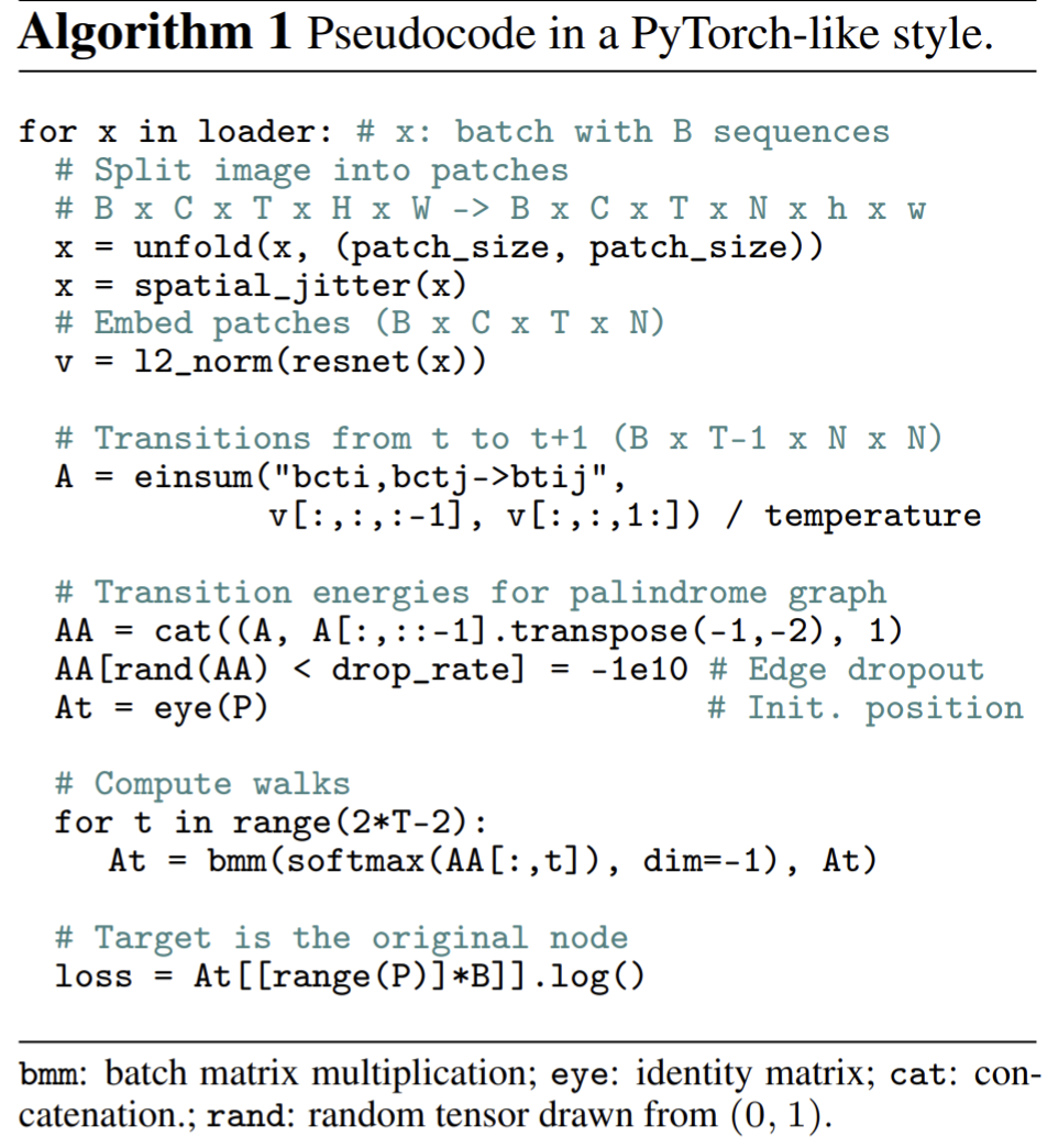
Paper 35: Spatially consistent representation learning

Codes: https://github.com/kakaobrain/scrl

Why

• Previous SSL methods are prone to overlook spatial consistency of local representations and therefore have a limitation in pretraining for localization tasks such as object detection.
• Aggresively cropped views used in existing contrastive methods can minimize representation distances between the semantically different regions of a single image.
• Contrastive SSL aims to obtain discriminative representations based on the semantically positive and negative image pairs.
• Most exisiting contrastive methods explot consistent global representations on a per image basis, they are likely to generate inconsistent local representations with respect to the same spatial regions after image transformations.
  • Lead to performance degradation on localization tasks based on spatial representations.
• Similar previous work
  • SwAV: introduce cluster assignment and swapped prediction, also propose multi-crop where they compare multiple smaller patches cropped from the same image, but substantially different in that the spatial consistency on the feature map is not directly considered.
  • BYOL removes the necessity of negative pairs and have shown to be more robust against changes in batch size.
  • SSL methods to leverage geometric correspondence are limited to dense representation irself that comes with object structure learning.

Goal

• Propose SCRL (spatially consistent representation learning) for multi-object and location-specific tasks.
• Devise a new SSL objectIve that tries to produce coherent spatial representations of a randomly cropped local region according to geometric translations and zooming operations.
• SCRL can possibly sample infinite number of pairs by pooling the variable-sized random regions with bilinear interpolation. VADeR is a specific instance of their methods where the sizes of the pooled box is fixed to a single pixel without a sophisticated pooling technique.

How

• From a positive pair of cropped feature maps, apply RoIAlign to the respective maps and obtain equally-sized local representations. Optimize the encoding network to minimize the distance between these two local representations. Adpat BYOL learning framework.

Spatially consistent representation learning

• Use two network, the online network parameterized by \(\theta\) and target network parameterized by \(\xi\). The target network provides the regression target to train the online network while \(\xi\leftarrow\tau\xi+(1-\tau)\theta\) (an exponential moving average with a decay parameter \(\tau\)).
• \(\mathbb{T}_1,\mathbb{T}_2\) denote two sets of image augmention strategies and then generate two augmented views \(v_1 =t_1(I),v_2=t_2(I)\). Then \(v_1,v_2\) are respectively fed into the two encoder networks \(f_\theta,f_\xi\) (without GAP layer) to obtain spatial feature maps \(m_1,m_2\).
• To find spatial correspondence, first find the intersection regions, use IoU to reject a candidate box.
• Then randomly sample an arbitrary box \(B=(x,y,w,h)\) in intersection region, the box has to be translated to the coordinates in each view, denoted as \(B_1,B_2\).
  • Though the size, location, and internal color of each box may be different for each views, the semanttic meaning in the cropped box area does not change between \(B_1,B_2\).
  • The box are rectangular box, and to map one box to another box after geometrical transformations, exclude certain affine transformations such as shear operations and rotations.
  • To obtain the equally-sized local representations from both boxes, crop the corresponding sample regions, called RoI, on the spatial feature maps and locally pool the cropped feature maps by \(1\times 1\) RoIAlign.
  • Sample \(K\) boxes on a given spatial feature map, one image can generate multiple pairs of local representations \(p_i^k\), where \(i\) denotes the view (\(i=1,2\)), \(k\) is the number of sampled boxes.
• In the online network (view 1), then perform the projection from \(p_1^k\) to get \(z_1^k\), followed by the prediction \(q_\theta(z_1^k)\), and the target network gets \(z_2 ^k\).
• The spatial consistency loss is MSE between the normalized prediction \(\bar{q_\theta(z_1^k)}=\frac{q_\theta(z_1^k)}{\|q_\theta(z_1^k)\|^2}\)and the normalized target prediction \(\bar{z_2^k}=\frac{z_2^k}{\|z_2^k\|^2}\).
  • To symmetrize the loss, also feed \(v_2\) to the online network and \(v_1\) to the target network respectively.
• use resnet as the backbone.

Paper 36: Spatiotemporal contrastive video representation learning

Codes: https://github.com/tensorflow/models/tree/master/official/

Why

• Traditional hand-crafted local invariant features for images have their counterparts in videos.
• The long-standing pursuit after temporal cues for self-supervised video representation learning has left selfsupervision signals in the spatial subspace under-exploited for videos.
• Simply applying spatial augmentation independently to video frames actually hurts the learning because it breaks the natural motion along the time dimension
• a pair of positive clips that are temporally distant may contain very different visual content, leading to a low similarity that could be indistinguishable from those of the negative pairs.
• The recent wave of contrastive learning shares a similar loss objective as instance discrimination.

Goal

• Propose CVRL (contrastIve video representation learning) to learn spatiotemporal visual representations from unlabeled videos.
• There are two augmented clips used for contrastive learning, augmented by their proposed temporally consistent spatial augmentation method and sampling-based temporal augmented method.

How

• construct positive pairs as two augmented video clips sampled from the same input video.
• CVRL is more effective with larger networks.

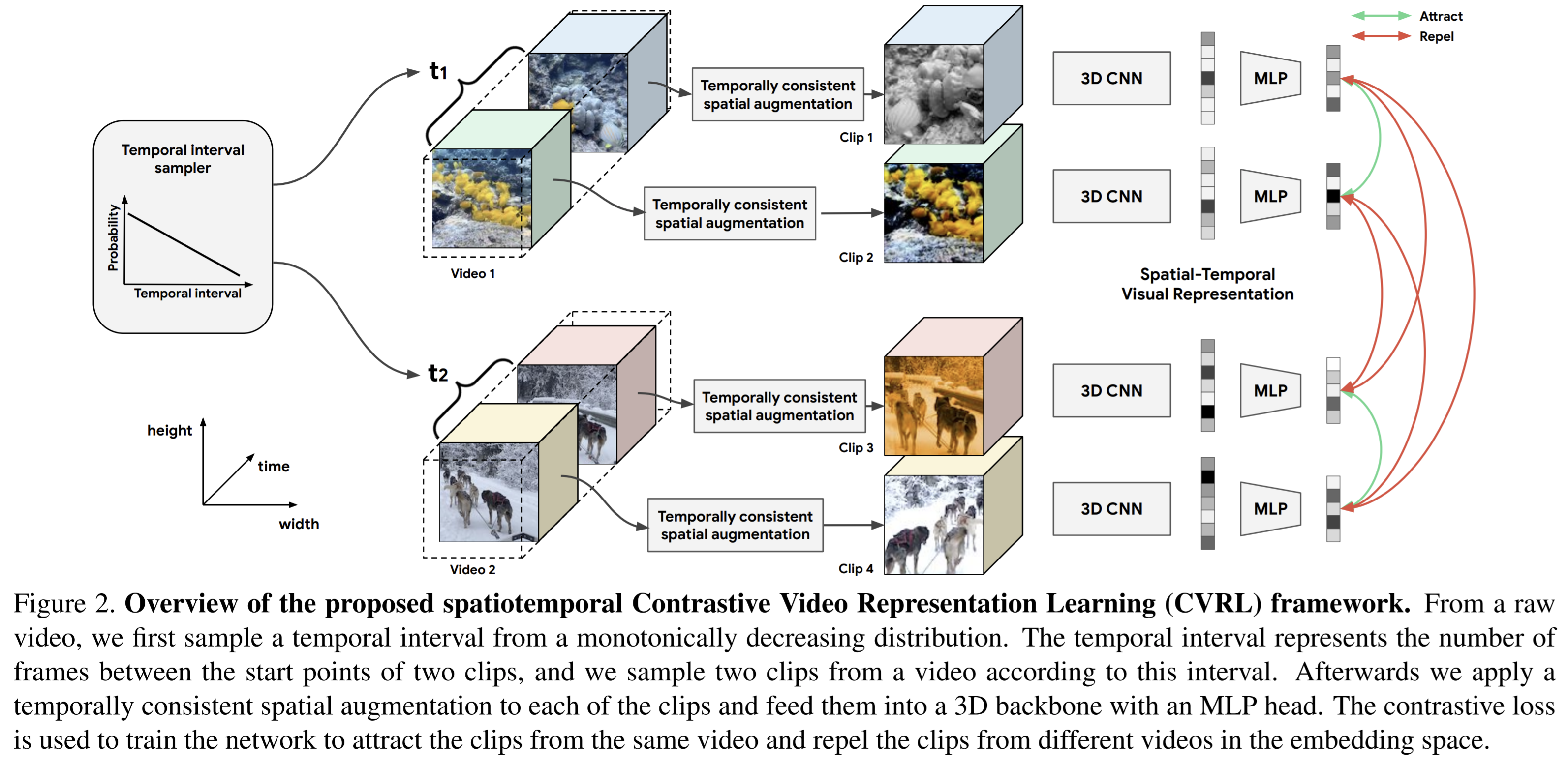
Video representation learning framework

• Use InfoNCE loss, which allows the postitive pair \((z_i,z_i')\) to attract mutually while they repel the other items in the mini-batch.
• Components: An encoder maps an input video clips to its representation \(z\), spatiotemporal augmentations to construct positive pairs \((z_i,z_i')\) and the properties they induce, and methods to evaluate the learned representations.

Video encoder

• Encode a video sequence using 3D-ResNets as backbones.
  • Only two changes on original 3D-ResNets: the temporal stride of 2 in the data layer, and the temporal kernel size of 5 and stride of 2 in the first CNN layer.
  • The video representation will be a 2048-dimensional feature vector.
• The add a multi-layer projection head (MLP) onto the backbone to obtain the encoded 128-dimensional feature vector \(z\).
• During evaluation, the MLP is dropped.

Data augmentation

• Temporal augmentation: The main motivation is that two clips from the same video would be more distinct when their temporal interval is larger.

  • If sample temporally distanct clips with smaller probabilities, the contrastive loss would focus more on the temporally close clips, pulling their features closer and imposing less penalty over the clips that are far away in time.==> aligning lower sampling probability on larger temporal intervals.
  • Steps: First draw a time interval \(t\) from a distribution \(P(t)\) over \([0，T]\), then uniformly sample a clip from \([0，T-t]\), followed by the second clip which is delayed by \(t\) after the first.
  • The descreasing distributions generally perform better than the unifom or increasing ones.

• Spatial augmentation: With fixed randomness across frames, the 3D video encoder is able to better utilize spatiotemporal cues.

  

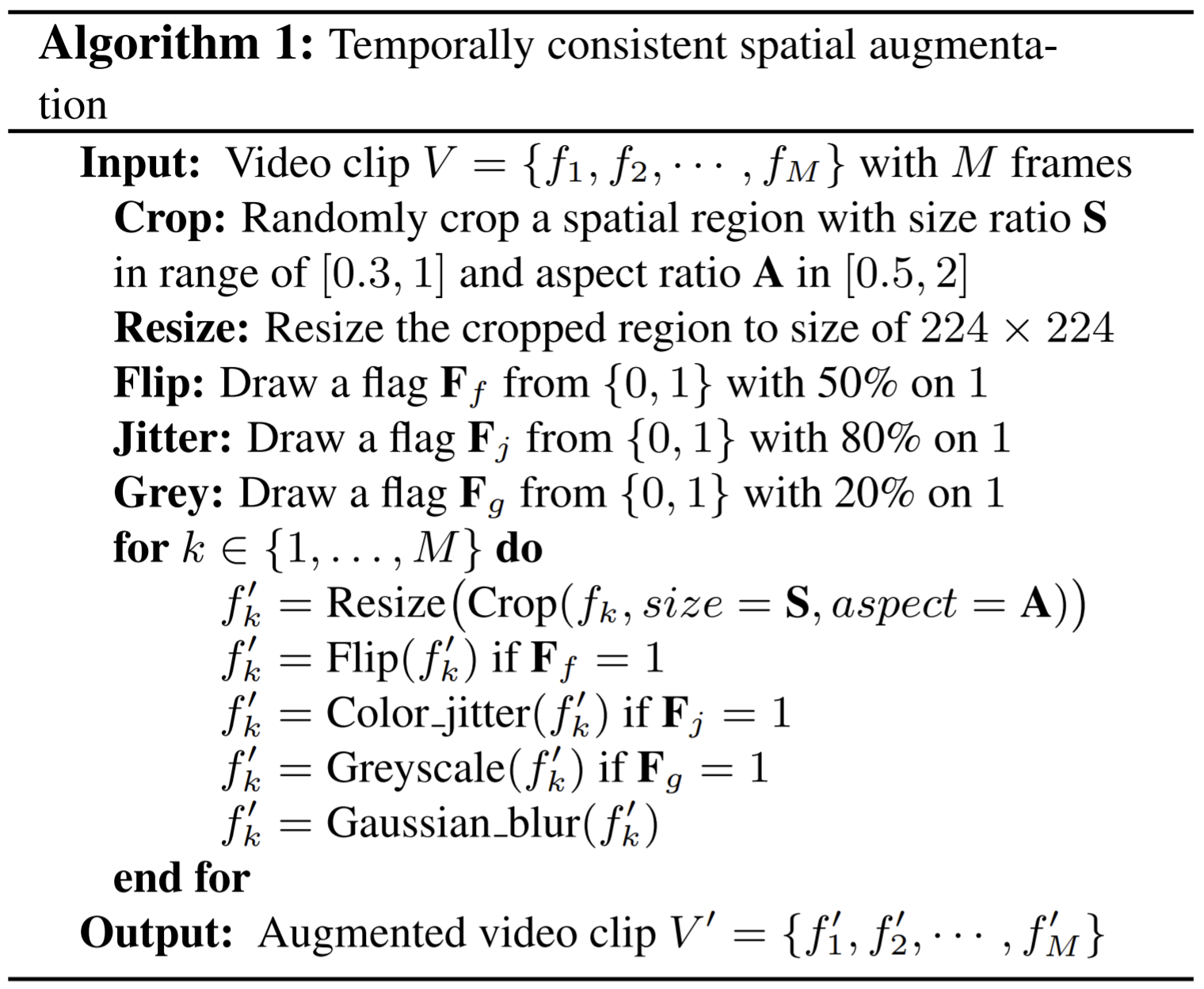
Evaluation

• evaluate the learned video representations by fixing the weights in the pre-trained video encoder and training a linear classifier on top of it.

Paper 37: SportsCap: Monocular 3D Human Motion Capture and Fine-grained Understanding in Challenging Sports Videos

Codes: https://github.com/ChenFengYe/SportsCap

Why

• Most existing action understanding solutions are limited to the pure high-level action assessment, where the abundant 3D motion capture information of sub-motions has been ignored.
• Previous methods on pose and shape estimation do not consider rich semantic information embedded in sports, and the structure constraints within sub-motions.
  • They use the underlying semantic and ordering rules in sport to reduce the complexity of the problem, and use PCA to capture the similarities of poses in each sub-motion and constrain estimated poses in reasonable forms.
  • Previous methods rely on 2D poses under-estimate the complex sports actions.
• Action parsing
  • Competitive sports are a mixture of long and short dynamics.
  • Approaches rely on joint motions ignore the patterns of the human body in certain activities.
• Dataset: To their knowledge, the SMART dataset is the only one that provides the fine-grained semantic labels, 2D ad 3D annotated poses, and assessment information.

Goal

• Monocular 3D Human Motion Capture on sports videos, use the semantic and temporally structured sub-motion prior in the embedding space. Propose a motion embedding module to recover both the implict motion embedding and explicit 3D motion details via a corresponding mapping function and a sub-motion classifier.
• reconstruct both the 3D human motion and the corresponding fine-grained action attributes from monocular professional sports video.
• The approach will provide sub-actions, action types and rotation angles .

How

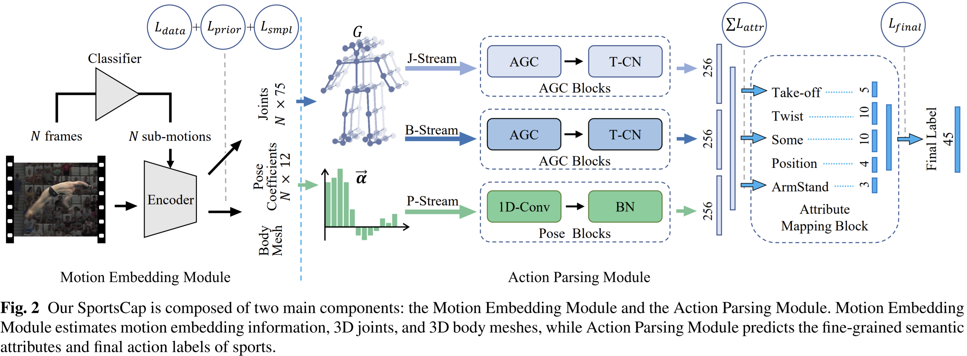
• The fine-grained semantic action attributes are predicted by ST-GCN, use both the original motion embedding stream and the recovered 3D detailed motion stream of the whole video clip.
• The model comprises of two modules
  • Motion embedding module: Use PCA to extract embedding prior, the estimate the per-frame motion embedding parameters (pose, shape) so as to recover the 3D motion details. The embedding module consists of a sub-motion classifier (WS-DAN) , a CNN encoder to regress the embedding and the mapping function from the embedding space to the 3D motion output.
  • Actions parsing module: use ST-GCN, input both the implicit pose embedding and the explicit 3D joints. Finally map the predicted attributes to the final action label by a semantic attribute mapping block.

Motion embedding and capturing

• Split one action into sub-motions. In each sub-motion, poses exhibit high resemblance across athletes.
• The sub-motion classifier is WS-GAN.
• Then use SMPL (skinned multi-person linear model) to build the motion embedding space, which represents the pose parameters as \(\theta\).
  • Use pose coefficient \(\boldsymbol{\alpha}\) to leverage the rich semantic and temporally structural prior of sub-motions in the motion embedding space. \(\boldsymbol\theta=\sum\limits_{k=1}^K\alpha_k\boldsymbol{b}_k^m+\boldsymbol{a}^m\), where \(\boldsymbol{a}^m\) is the mean of pose parameters, and \(\boldsymbol{\alpha}\) are the pose coefficients.
• Then use PCA on pose parameters \(\boldsymbol{\theta}\), the \(\boldsymbol{b}_k^m\) in above are PCs, and \(\boldsymbol{a}^m\) denotes the mean, and \(\alpha\) means the coefficient assigned by std.
• The module consists of a resnet-152 encoder followed by two FCC to regress the pose coefficients \(\boldsymbol{\alpha}\) and then reconstruct joint positions
  • 
  • Use this network to estimate pose coefficients, shape parameters and camera parameters from images. Then recover 3D human body meshes from estimated pose and shape parameters of SMPL.

Action parsing

• Tasks include inferring semantic meaningful labels and the action number (code ) from sports videos.

• Use SAs (semantic attributes, are learnt by ST-GCN ) to represent the semantic meaningful label. The action number represents a valid combination of SAs.

  • SAs indicate the specific number of a motion (the number of frames for one type of motion?), like the rotation angle, take-off type and so on.

  • For one sequence, there maybe are many types of motions that intersect together?

    

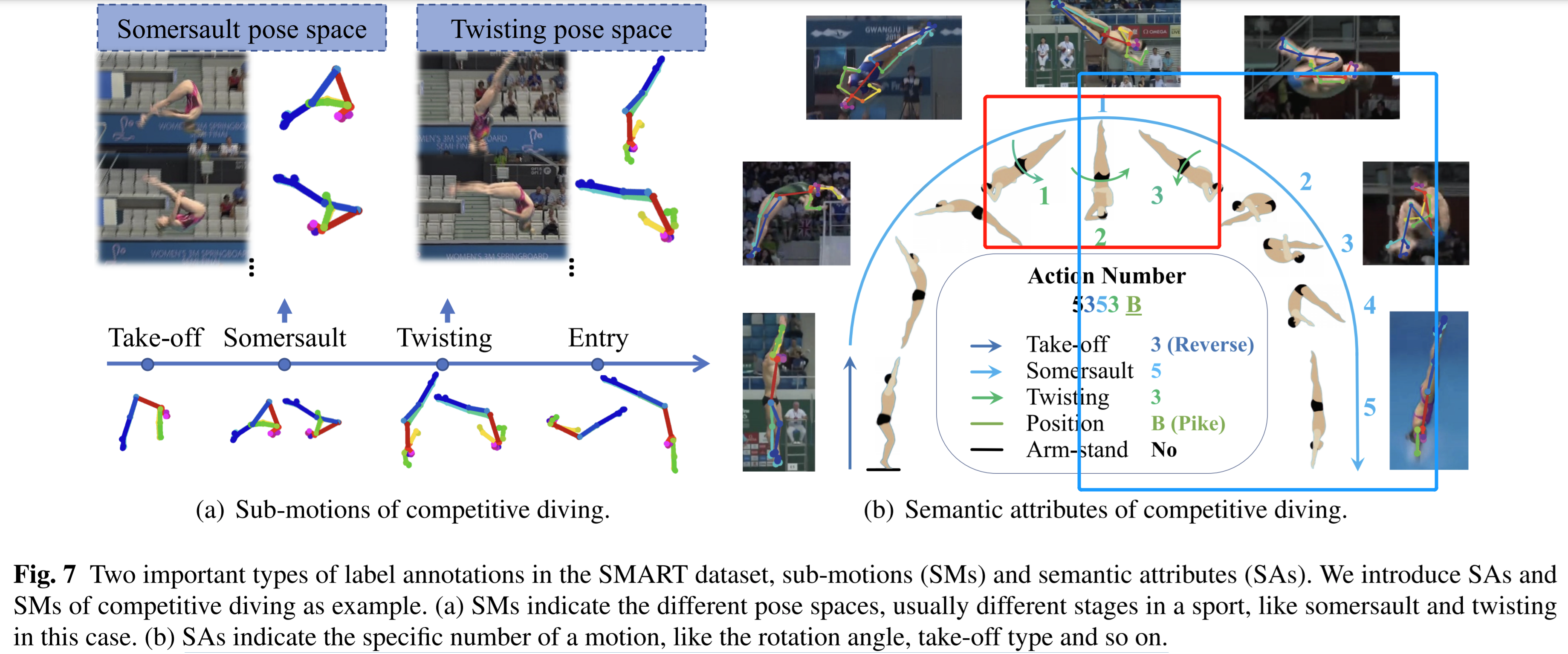
• ST-GCN for extract SAs.

  • J- and B-Stream use 2s-AGCN.
  • In P-stream, represent pose coefficients as a 1D vector and use 1DCNN with residual to generate features.

• Semantic attributes mapping block

  • Learn the mapping between the extracted ST features and the final action label.
  • Goal: partition the whole action sequence in terms of SAs, or to say how individual frames contribute to specific SAs.
  • Use two FCs to predict their contributions, then stack the resulting SAs and feed the results to another 2 layer FCs to infer the action number.

Multi-task training

• Loss for motion embedding module
  • The prior loss: \(\mathcal{L}_{prior}=\|\mathrm{W}(\bar{\alpha}-\hat{\alpha})\|_2\), where \(\bar{\alpha}\) is the mean of pose coefficients in training set, and \(\hat{\alpha}\) is the predicted pose coefficients.
  • The data loss: On 2D pose, \(\mathcal{L}_{data}=\|\mathrm{V(J-\hat{J})}\|_2\), where \(\mathrm{J}\) is the ground truth, and \(\hat{\mathrm{J}}\) is the estimated 2D joints, which are projected from estimated 3D points. \(\mathrm{V}\) denotes the visibility of the ground truth joint.
  • SMPL loss: \(\mathcal{L}_{smpl}=\|\theta-\hat{\theta}\|_2+\|\beta-\hat{\beta}\|_2\), where \(\theta,\beta\) are the supervision of pose/shape parameters.
  • The final loss is the combination of previously listed 3 losses.
• Loss for action parsing module
  • Use the cross-entropy between the predicted and the ground truth attributes.
  • The acion labeling task also use the cross-entropy loss.
  • The final loss in this module is the combination of three losses.
• Training strategy:
  • Stage 1: train a motion embedding module for each sub-motion independently and fix its parameters
  • Stage 2: Then train the action attribute prediction and label classification modules in the action parsing module jointly.
  • Stage 3: Fine tune the entire network using the combined losses from two modules.

Paper 38: SSAN: Separable Self-Attention Network for Video Representation Learning

Why

• Self-attention succeed in video representation learning due to its ability of modeling long range dependencies. Existing methods build the dependencies merely by the pairwise correlations along spatial and temporal dimensions simultaneously.
  • However, spatial correlations and temporal correlation represent different contextual information of scenes and temporal reasoning.
  • Learning spatial contextual information will benefit temporal modeling.
• Learning strong and generic video representations is still challenging.
  • Videos contain rich semantic elements within individual frames, but also the temporal reasoning across time.
  • The long-range dependencies among pixels cannot be well-cared by CNN.
  • RNN does, but sufferes from the high computation cost, and it cannot establish the direct pairwise relationship between positions regardless of their distance.
• The correlations from space and time represent different contextual information. The former often relates to scenes and objects, and the latter often relates to temporal reasoning for actions (short-term) and events (long-term).
  • Learning correlations along spatial and temporal dimensions together might capture irrelevant information, leading to the ambiguity for action understanding
  • Short-term dependencies should also be considered for capturing episodes of complex activities.
• Video learning networks
  • Mainly two branches for video learning architectures: 2D based methods and 3D based methods.
  • But 3D based methods suffer from the overhead of parameters and complexity, while 2D based methods need careful temporal feature aggregation.
• Action recognition
  • video classification, early works try to use 2D based methods to video, the 3DCNN are used. But huge computation cost.
  • 3D based methods always take several consecutive frames as input, so that videos with complex actions cannot be well handled.
  • 2D convolution networks with temporal aggregation achieve significant improvements.
• Self-attention
  • The full connections among pixels also introduces irrelevant information.
  • The 3D based self-attention can model long dependencies from space and time simultaneously, but such dependencies are first-order correlations which mainly capture the similarity between single pixels, not semantic-level correlations.
  • Non-local methods consider more on position-wise correlations but less on channel-wise correlations.
• Visual-language learning
  • VideoBERT: propose to use a visual-linguistic model to learning high-level features without any explicit supervision.
  • Sun et al.: use contrastive bidirectional transformer (CBT) to perform SSL for video representations.
  • UniViLM: propose a joint video and language pre-training scheme by adding generation tasks in the pre-training process.
  • These methods only focus on the training of the transformer encoder and decoder, while take the video networks as feature extractors.

Goal

• Propose separable self-attention (SSA) module, which models spatial and temporal correlations sequentially.
• The proposed SSA learn spatial self-attention firstly. The attention maps are then aggregated along temporal dimension and sent to temporal attention module.

How

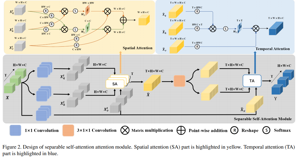
Self-attention in vision

• If videos \(X\) in \(T\) frames, in size \(H,W,C\), then reshape the embedding for query, key and value to size \(THW\times C,C\times THW,THW \times C\), respectively, denoted by \(X_q,X_k,X_v\).
• Then the attention map Y is \(Y=softmax(X_q\times X_k)\times X_v\) in size \(THW \times C\).
• Then it is transformed by \(1\times 1\times 1\) convolution and added back to the original query feature \(X\). \(Z=W_z(Y)+X\).

Separable Self-attention module

• The spatial and temporal attention are performed sequentially, so that temporal correlations can fully consider the spatial contexts. Second, sptial attention maps exploit as much context information as possible.
• First use 2D \(1\times 1\) convolutions to map input feature \(X\) into \(X_q,X_v,X_k\).
• After spatial attention, the 4D intermediate attention map \(\hat{X}\) (after spatial attention) is then transformed to temporal embeddings \(\hat{X}_q,\hat{X}_v\) using \(3\times1\times 1\) convolution. The temporal attention still use same \(X_v\) (same as what's used in spatial attention ).
• Spatial attention
  • Both position-wise and channel-wise attention, so two similarity matrices \(M_s,M_c\) are generated.
  • The final spatIAL maps for time \(t\) is \(\hat{X_t}=(M_s\times X_{v(s)}^t)+(M_s\times X_{v(c)}^t)\), and the intermediate attention map \(\hat{X}=Cat[\hat{X}_0,\cdots,\hat{X}_T]\).
• Temporal attention
  • \(3\times1\times 1\) convolution alloes temporal fusion on spatial attention maps and builds the short range correlations along temporal dimension.

Network architecture

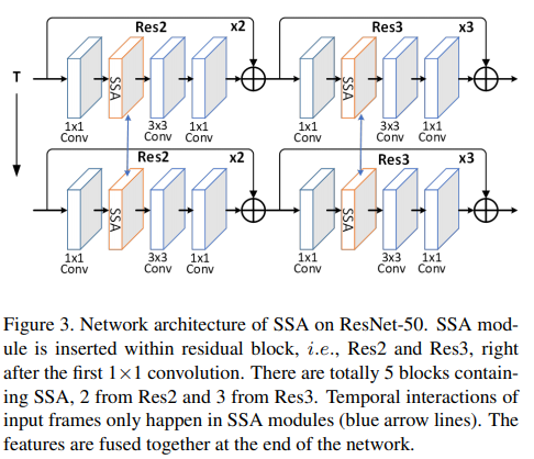
• Choose TSN as the baseline, insert SSA module into different layers to establish separable self-attention network (SSAN).

Paper 39: tdgraphembed: Temporal dynamic graph-level embedding

Codes: https://github.com/moranbel/tdGraphEmbed

Why

• Existing graph embedding methods focus on capturing the graph's nodes in a static mode and/or not model the graph in its entirety in temporal dynamic mode.
• To the best of their knowledge, the novel task of embedding entire graphs into a single embedding in temporal domains has not been addressed yet.
• Graph representation learning on Static graph context:
  • Matrix factorization: like SVM, LLE, decompose the Laplacian or higher-order adjacency matrix to produce node embedding that preserves the distance between ndoes.
  • Random walk based methods: create random path over the graph and use word2vec-like architecture for the node embedding task
  • Deep learning based methods: like autoencoders, GCN, GAEs
• Unsupervised graph embeddings
  • Graph2vec: embed the entire graph in a static mode and use an analogy between graphs and documents, take the rooted subgraphs around every node as the context terms that make up the document
  • Sub2vec, unsupervised, for arbitrary static subgraphs using gone random walk
  • UGraphEmbed: graph-level representation, the embeddings of two graphs preserve their graph-graph proximity based on GED measure.
  • But they encode the graph without considering the historical contexts.
• Temporal node/edge embedding methods
  • generate node embeddings at each time step of the graph using static embedding, and then align them to from a unified representation
  • DynGEM: use the learned embeddings from the previous graph to initialize the representation at current time.
  • Dyngraph2vec: recurrent layers to learn patterns over sequence of graphs.
  • They don't take the fact that the number of nodes changes over time into consideration.
  • DyRep: use two time scaling process that captures temporal node interactions ad topological evolution, but only supports the network's growth; DynamicTriad: analyze every two consecutive timesteps to create the embedding. ==> But not graph-level embedding.

Goal

• Temporal dynamic graphs, propose tdGraphEmbed to learn temporal graph-level embedding unsupervisedly, which is an extension of random walk that globally embed both the nodes of the graph and its representation at each step.

How

• The proposed method embeds the entire graph at timestamp \(t\) into a single vector \(G_t\). At each timestamp \(t\), it performs \(\gamma\) random walks of length \(L\) from each node in the graph. Then jointly learn the node embeddings \(v\) along with the entire graph embedding \(G_t\).
• The optimization becomes predicting a node embedding given the node's context in the random walks at time \(t\) of the graph and the vector \(G_t\).

Random walk

• Modeling each graph as a sequence of sentences, and then model the graph's sentences using random walks.
  • Denote a random walk initiated at node \(v_i\) as \(\mathcal{W}_{v_i}\). Then a random walk is a stochastic process with random variables \(\mathcal{W}_{v_i,1},\mathcal{W}_{v_i,2},\cdots,\mathcal{W}_{v_i,k}\) such that \(\mathcal{W}_{v_i,k+1}\) is a node chosen at random from the neighbors of node \(W_{v_i,k}\).
  • Implement a second order random walk with a return parameter \(p\) and an in-out parameter \(q\) to guide the walk.
    • Use \(p,q\) to adjust the transition probability \(\alpha_{pq}(u,x)\) from node \(u\) to some node \(x\): \(\alpha_{pq}(u,x)=\begin{cases}\frac{1}{p} & if d_{ux}=0\\1 & if d_{ux}=1\\ \frac{1}{q}& if d_{ux}=2\end{cases}\), where \(d_{ux}\) indicates the distance between node \(u\) and node \(x\).
    • Then this node2vec can bias the random walk closer or further away from the source node, creating different embedding types.
    • Precisely, \(p<q\) biases the random walk to noes closer to each other, then nodes from the same cluster to be embedded closer and nodes from different regions to be embedded further away; \(p>q\) biases the random walk to embed nodes of the same graph characteristics closer together while others are embedded further away.
• Then the goal is to estimate the likelihood of observing \(G_t\) in its entirety given all random walks at time \(t\), defined as \(Pr(G_t|(\mathcal{W}_{v_1},\mathcal{W}_{v_2},\cdots,\mathcal{W}_{v_k}))\).

Framework

• Each node is initialized by \(\gamma\) random walks of length \(\mathcal{L}\).

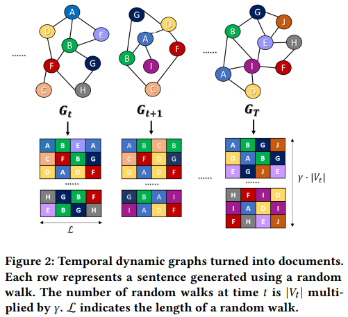
• After the step shown in figure 2, the goal is to predict the next node in a random walk. Take context nodes (sampled from a sliding window \(\omega\) over random walks), also known as nodes in the neighborhood of the root node, and denote as \(N_s(v_i^t)\).

• To learn the representation map \(\phi\) that maps a given node and graph to a \(d\)-dimensional space, then maximize \(\log p(v_i^t|N_s(v_i^t),G_t)\) for each node in \(V_t\), which is defined by softmax. \(\log p(v_i^t|N_s(v_i^t),G_t)=\frac{\exp (\phi(v_i^t)\cdot h)}{\sum_{j\in V_t}\exp(\phi(v_j^t)\cdot h)}\), where \(h\) is the combination of mapped node embedding and mapped graph embedding \(G_t\), and map means \(\phi\).

• The graph’s time index can be thought of as another node which acts as a memory for the global context of the graph.

• Finally, the objective is

  

Tips

• To decrease computation cost, use negative sampling for the denominator of softmax.
• 

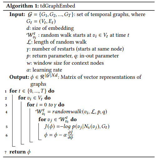
Paper 40: Videomoco: Contrastive video representation learning with temporally adversarial examples

Why

• The evolution of contrastive learning heavily focuses on feature representations from static images while leaving the temporal video representations less touched.
  • Large scale video data is difficult to store in memory.
  • Attempts on unsupervised video representation learning focus on proposing pretext tasks related to a sub-property of video content.
• MoCo treats the contribution of keys from the queue only based on their representation. But in fact, the longer the keys in the queue, the more different their representations are compared to those of the current input samples.

Goal

• An extension of MoCo to learn video representation unsupervisedly.
• Two modifications given a video sequence as a sample
  • Introduce a generator to drop out several frames from the sample temporally.==> by dropping during adversarial training, force the input sample to train a temporally robust encoder.
  • Use temporal decay to model key attenuation in the memory queue when computing contrastive loss. As the momentum encoder updates after keys enqueue, the representation ability of these keys degrades when we use the current input sample for contrastive learning.
• VideoMoCo utilizes color information and performs instance discrimination without bringing empirical pretext tasks.

How

• Introduce adversarial learning to improve the temporal robustness of the encoder
  • Use a generator to adaptively drop out several frames
  • And the dropped samples are sent to discriminatory for differentiating.
  • After adversarial training, only D is kept to extract temporally robust features.
• The sample after dropping out some frames is then taken as a query sample and perform contrastive learning with keys in the memory queue.
  • Model the degradation of keys by proposing a temporal decay. If a key stays longer in the queue, its contribution is less (manipulated by the decay).

MoCo

• The contrastive loss of MoCo \(L_q=-\log \frac{\exp (q\cdot k_+/\tau)}{\sum\limits_{i=0}^K\exp(q\cdot k_i/\tau)}\), which tends to classify \(q\) as \(k_+\). The query \(q\) is the representation of an input sample via the encoder network, while the keys \(k_i\) are the representations of the other training samples in the queue.
• The queue follows FIFO scheme. Denote the parameters of an encoder as \(\theta_q\) and those of a momentum encoder as \(\theta_k\). The momentum encoder is updated as \(\theta_k\leftarrow m\theta_k+(1-\theta)\theta_q\), where \(m\) is a momentum coefficient.
• For VideoMoCo, give an input video clip with a fixed number of frames, the model sent it to a generator G and the encoder D to produce \(q\). Meanwhile, reweigh \(\exp(q\cdot k_i/\tau)\) by \(t^i,t\in(0,1)\).

Temporally adversarial learning

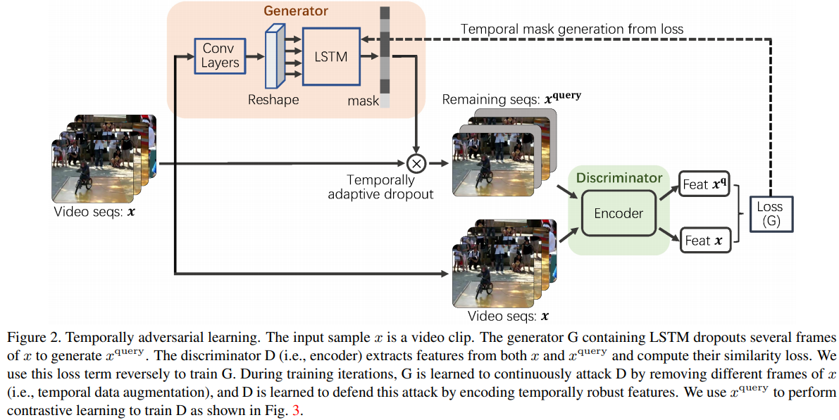
• G, consisting of ConvLSTM, takes \(x\) as input and produces a temporal mask. The mask will help drop out \(25\%\) of the frames.
• Regard the encoder of MoCo as the discriminator D, and take \(X^{query},x\) as the input of D.
• Tips for training: Initially, we train D without using G and only use contrastive learning. When D is learned to approach a semi-stable state, we train D by involving G. We empirically observe that utilizing adversarial learning at the initial stage makes D difficult to converge.

Temporal decay

• For a key \(k_i\) in the queue, set its corresponding temporal decay as \(t^i\) where \(t\in(0,1)\), and \(i\) gradually increases by 1 and \(t^i\) decreases correspondingly.

• Then with \(t^i\), the real loss function for the discriminator D is

  

Visualization

• After obtaining classification scores, use entropy to measure the classifier's confidence when making the prediction. A high entropy value means the classifier is more uncertain on making the current predictions.
• Even though both MoCo and VideoMoCo can resist temporally occluded video sequences, the feature representation of MoCo has become very fragile while that of VideoMoCo does not degrade significantly.
• The features learned from VideoMoCo attend the network to the temporal motions.
  • How to calculate attention maps?

Paper 41: Visual Relationship Forecasting in Videos

Why

• Current efforts mostly focus on detecting the object interactions based on observation rather than reasoning about the spatiotemporal connections among predicates.
• VRF requires additional spatiotemporal modeling among time series. This task emphasizes the importance of visual relationship reasoning.
• Future prediction
  • generating future frames: usually generative models
  • predicting future labels or states: multiple methods, VRF can be classified into this group. It performs forecasting on the unknown future frames, and it focuses on the relationship forecasting among a specific pair of .

Goal

• Deal with object interactions in unknown future. Propose VRF (visual relationship forecasting, a new task) in videos to explore the prediction of visual relationships in a reasoning manner.
  • Formally, given a subject-object pair with \(H\) existing frames, it aims to predict their future interactions for the next \(T\) frames without visual evidence.
  • Propose a graph convolutional transformer (GCT) framework, which captures both object-level and frame-level dependencies by ST-GCN (object-level ) and transformer (frame-level) .

How

• Propose GCT

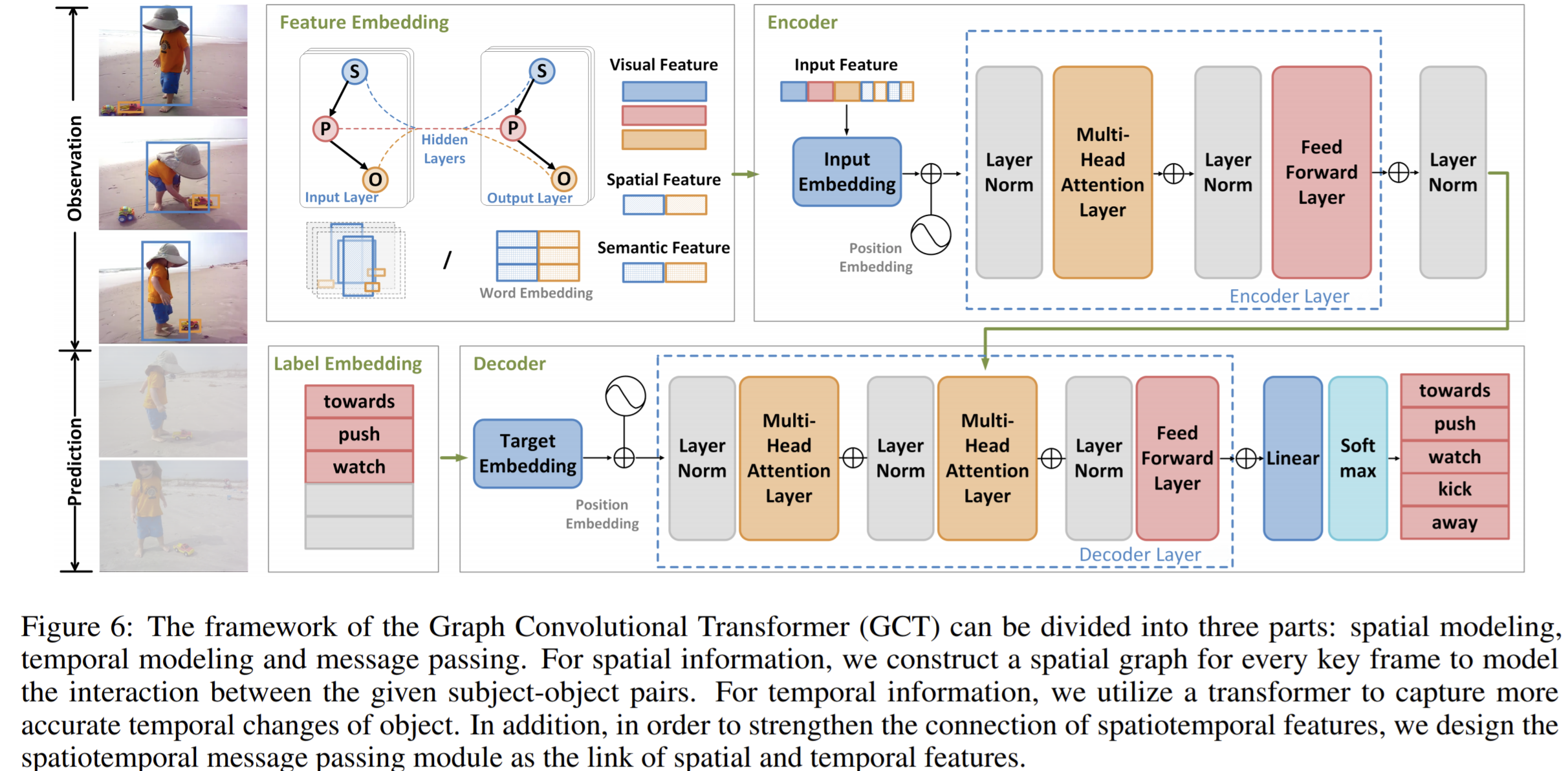
Framework

• GCT can be divided into three parts: feature representation, object-level reasoning, and frame-level reasoning.
• In feature representation module, use visual feature, semantic feature and spatial features. For spatial reasoning, a spatial graph is constructed for every key fame and the corresponding GCN is taken to model the interactions between the given pairs.
• Then, use a multi-head transformer for frame-level reasoning.

Feature representation

• Visual features: Use the bounding boxes of one instance, \(b_s,b_{so},b_o\) indicate the subject, predicate and object bounding box. Use Inception-ResNet-V2 as the backbone and extract the features of these bounding boxes from the fully connected layers.
• Spatial features: Get the relative spatial feature of bounding boxes, adopt the idea of box regression.
  • \(\Delta(b_i,b_j)\) denote the box delta that regresses the bounding box \(b_i\) to \(b_j\), \(dis(b_i,b_j)\) and \(iou(b_i,b_j)\) denote the normalized distance and IoU between \(b_i,b_j\), and the union region of \(b_i,b_j\) is denoted as \(b_{ij}\).
  • The relative spatial location of subject and object can be defined as: \(l_{ij}=[\Delta(b_i,b_j);\Delta(b_i,b_{ij});\Delta(b_j,b_{ij});iou(b_i,b_j);dis(b_i,b_j)]\).
• Semantic features: Adopt a semantic embedding layer to map the object category \(c\) into word embedding \(s\).
  • The parameters of object categories are initialized with the pre-trained word representations such as word2vec.

Object-level reasoning

• The spatiotemporal graph \(\mathcal{G}=\{\mathcal{V}_o,\mathcal{V}_p,\mathcal{E}\}\) is constructed, containing an object node set \(\mathcal{V}_o\), a predicate node set \(\mathcal{V}_p\), and an edge set.
  • \(v_i\in \mathcal{V}_o\) represents an object bounding box \(b_i\) in a video fame, corresponding with object category \(c_i\).
  • \(v_i\in \mathcal{V}_p\) represents a predicate bounding box \(b_i\) in a video fame, corresponding with predicate category \(c_i\).
  • There is an edge between an object node and a predicate node, but no links between two object nodes.
  • The objects and predicate nodes in the key frames at different moments are all included in the corresponding node set
• Then, perform GCN on the built graph.

Transformer for temporal modeling

• The encoder layer encode the object-level features outputed by GCN, spatial features and semantic features into continuous representations. The encoder will output \(E\) as the feature representation.
• The decoder will use multi-head attention on \(E\), with two multi-head attention layers.
• The final decoder embedding is sent to a FC layer and a softmax to get the final prediction.
• Cross-entropy for optimization.

Paper 42: Wasserstein embedding for graph learning

Codes: https://github.com/navid-naderi/WEGL

Why

• The research on kernel approaches, perhaps most notably the random walk kernel and the WL kernel, remains an active field of study.

• Recent works

  • One propose a node embedding based on WL kernel, and combine the resulting node embeddings with the Wassertein distance.
  • Previous works all suffer from graphs in huge size.
    • On the GCN side, optimization is challenging.
    • On the graph kernel side, calculating the matrix of all pairwise similarities can be a burden.
  • Graph kernels
    • The shortest-path kernels
    • The graphlets and WL subtree kernel.
    • Others like kernel methods using spectral approaches, assignment-based approaches, and graph decomposition algorithms.

• Wassertein distance

  • Due to Brenier's theorem , for absolutely continuous probability measures \(\mu_i,\mu_j\), the 2-wassertein distance can be equivalently obtained from

    

  • The mapping \(f\) is referred to as a transport map, and the optimal transport map is called the Monger map.

  • But pairwise calculation of the Wassertein distance could be expensive.==> The linear optimal transportation framework between the probability measures to define a Hilbertian embedding, in which the \(\ell_2\) distance provides a true metric between the probability measures that approximates \(\mathcal{W}_2\).

Goal

• learn graph-level representations, propose WEGL(wassertein embedding for graph learning). Define the similarity between graphs as a similarity function between their node embedding distributions. And use wassertein distance to measure the dissimilarity between node embeddings of different graphs.
• WEGL calculates Monger maps from a reference distribution to each node embedding and, based on these maps, creates a fixed-sized vector representation of the graph.
• WEGL embeds a graph into a Hilbert space, where the \(\ell_2\) distance between two embedded graphs provides a true metric between the graphs that approximates their 2-Wassertein distance.

How

Linear Wassertein embedding

• The probability distributions are mapped to the tangent space with respect to a fixed reference distribution. The framework below is for isometric Hilbertian embedding of probability measures such that the Euclidean distance between the embedded images approximates \(\mathcal{W}_2\).
• By define \(\phi(\mu_i)\) as a function of Jacobian equation \(p_0\), the identity function \(id(z)=z\) and the Monge map \(f_i\), where \(f_i=\arg\min_{f\in MP(\mu_0,\mu_i)\int_{\mathcal{Z}}\|z-f(z)\|^2d\mu_0(z)}\). \(\phi(\mu_i)\) provides an isometric embedding for probability measures.
  • \(\|\phi(\mu_i)-\phi(\mu_0)\|_2=\|\phi(\mu_i)\|_2=\mathcal{W}_2(\mu_i,\mu_0)\), with \(\phi(\mu_0)=0\)
  • \(\|\phi(\mu_i)-\phi(\mu_j)\|_2\approx\mathcal{W}_2(\mu_i,\mu_j)\).
• Since \(\phi(\mu_i)\) provides a linear embedding for the probability measures, it's called the linear Wassertein embedding. It can also be thought as the RKHS embedding of the measure \(\mu_i\).
• For the discrete distributions , the Monge coupling is used.
• 
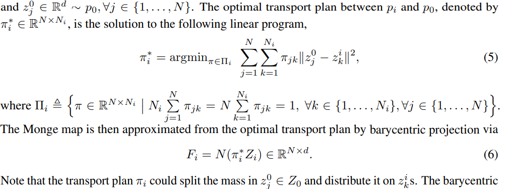
• The Monger map is the approximated from the optimal transport plan by barycentric projection via \(F_i=N(\pi_i^*Z_i)\in\mathbb{R}^{N\times d}\), and \(\phi(Z_i)=(F_i-Z_0)/\sqrt{N}\in\mathbb{R}^{N\times d}\).
  • Since the barycentric projection, \(\phi(\cdot)\) is only pseudo-inverible.

WEGL

• Applying optimal transport to measure the dissimilarity between two graphs, the entire embedding for each graph \(G_i\), is obtained by composing \(\phi(\cdot)\) and \(h(\cdot)\),i.e., \(\psi(G_i)=\phi(h(G_i))\) where \(h\) is an arbitrary node embedding process.

  

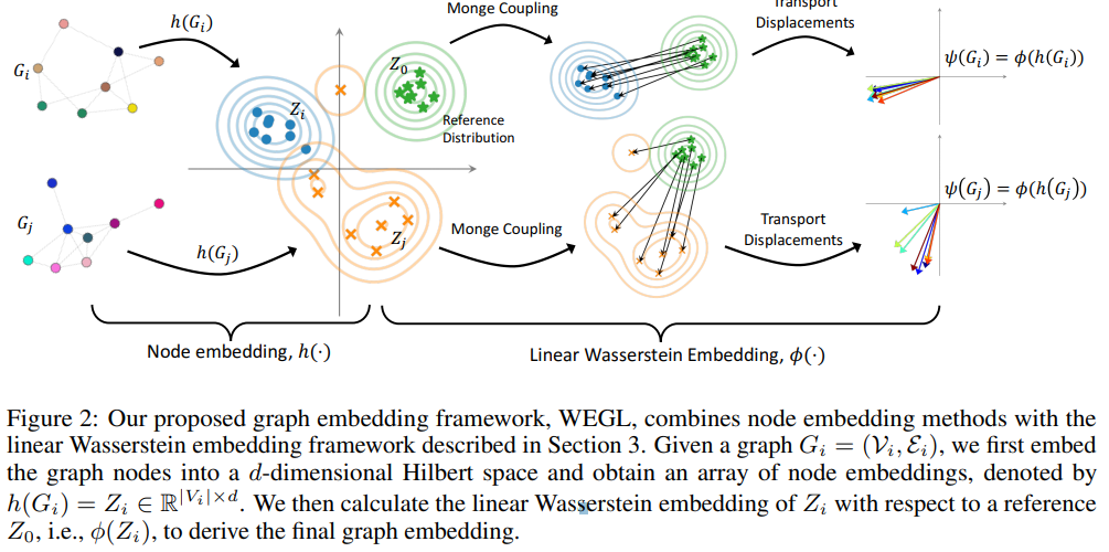
• Node embedding

  • They use a similar non-parametric propagation/diffusion-based encoder as in here .

  • Precisely, given node features \(\{x_v\}_{v\in\mathcal{V}}\) and scalar edge features \(\{w_{uv}\}_{(u,v)\in\mathcal{E}}\), \[ x_v^{(l)}=\sum\limits_{u\in\mathcal{N}_v\cup\{v\}}\frac{w_{uv}}{\sqrt{\deg(u)\deg(v)}}\cdot x_u^{(l-1)},\forall l\in\{1,\cdots,L\},\forall v\in\mathcal{V}\\ z_v=g(\{x_v^{(l)}\}_{l=0}^L\}) \]

where \(g(\cdot)\) is a local pooling process on a single node, \(z_v\) is the result embedding for each node.

• Calculation of the reference distribution
  • Use k-means on \(\cup_{i=1}^MZ_i\) with \(N=\lfloor\frac{1}{M}\sum\limits_{i=1}^MN_i\rfloor\) centroids.
  • Or one can calculate the Wassertein barycenter of the node embeddings or simply use \(N\) samples from a normal distribution.

Paper 43: Anomaly Detection in Video via Self-Supervised and Multi-Task Learning

Codes: https://github.com/lilygeorgescu/AED-SSMTL. Need to fill the form firstly.

Why

• Previous work on anomaly detection
  • Prediction based, and reconstruction error as the clue.
  • Reconstruction error
  • The dissimilarity between patches in Siamese network.
  • Eliminate the reliance of anomaly detection on context and form the problem as HAR.
• Addressing anomaly detection through a single proxy task is suboptimal.

Goal

• anomalous event detection in video at object-level.
• Use 3DCNN on three pretext tasks and one distillation task. The tasks are : discrimination of forward/backward moving objects (arrow of time), discrimination of objects in consecutive/intermittent frames, reconstruction of object-specific appearance information. The distillation task is based on teacher-student mechanism.

How

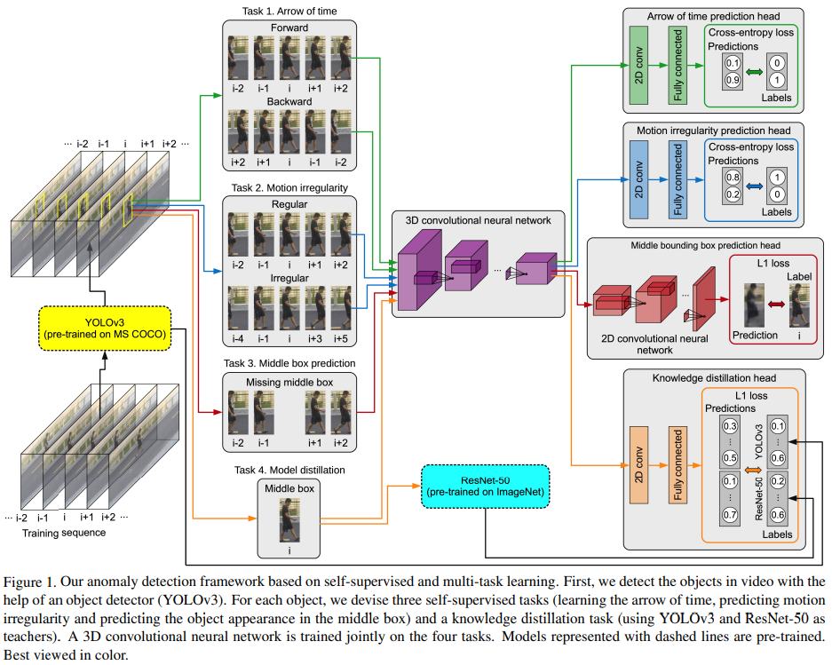
• YOLOv3 and ResNet-50 as teachers.
• Data preparation: use YOLOv3 to generate an object-centric temporal sequence by simply cropping the corresponding bounding box from frames.
• The anomaly score is the average scores predicted fro each task.
• Four tasks share the 3DCNN together, but each task has its prediction head.

Task 1: arrow of time

• For one sequence, create a forward and a backward sample, then train.
• Use cross-entropy

Task 2: motion irregularity

• Use one consecutive clip and the other is composed of the centric frame and other sampled frame, with a step sampled from \(\{1,2,3,4\}\).
• Use cross-entropy

Task 3: middle bounding box prediction

• Use the sequence with the centric frame missing and try to predict the missing one.
• Use L1 loss.

Task 4: model distillation

• Resnet 50 pretrained on ImageNet and YOLOv3 pretrained on MS COCO as the teacher who gives the GT, first YOLOv3 to get the middle box and the prediction \(Y_{yolo}\), then input the middle box to resnet 50 to get the prediction \(Y_{res}\), these two predictions are concatenated together as the GT.
• The shared 3DCNN is the student who use the features before input in resnet 50.
• Use L1 loss.

Joint loss

• Summation of the four loss, but the 4th loss is weighted summed to regulate the importance of the knowledge distillation task.

Inference

• For an object, the abnormal score is the average from four tasks. The pixel-level anomaly map uses a 3D mean filter. For a certain frame, it is taken as the maximum score in the corresponding anomaly map. The final frame-level anomaly scores are obtained by a temporal Gaussian filter.
• The failures of YOLOv3 are translated into false negatives.
  • By fusing the frame-level and object-level anomaly scores.

Paper 44: Exponential Moving Average Normalization for Self-supervised and Semi-supervised Learning

Codes: https://github.com/amazon-research/exponential-moving-average-normalization

Why

• The BN used in both teachers and students can lead to
  • Cross-sample dependency: caused by the intrinsic property of BN where the output of a sample is dependent on all other samples in the same batch. To solve this, some use layer normalization, MoCo designs ShuffleBN where a mini-batch uses BN statistics from other randomly sampled mini-batch. SimCLR and BYOL use Synchronized BN.
  • Model parameter mismatch: parameters in a teachers comes from the student in previous iterations, while the batch-wise BN statistics are instantly collected at current iteration, which will lead to potential mismatch between the model parameters and the BN statistics in the parameter space.
• Normalization
  • BN introduces some issues: the large batch sizes for accurate statistics, mismatch between how BN is used during training and inference
  • Other normalization
    • Layer normalization (LN) : along the channel and spatial dimension.
    • Instance normalization (IN): along only the spatial dimension
    • Group normalization (GN): similar to LN, divides the channels into groups.
    • MABN: similar with EMAN, but focus on the stability of small batch size training and updates its statistics inside a single network.
    • ShuffleBN: a minibatch uses BN statistics from other randomly sampled minibatch.

Goal

• Propose a plug-in replacement for BN called EMAN (exponential moving average normalization), for the improvement of student-teacher mechanism.
• EMAN in the teacher side updates statistics by exponential moving average, from the BNN statistics of the student. This design reduces the intrinsic cross-sample dependency of BN and enhances the generalization of the teacher.

How

• The EMAN statistics \(\mu,\sigma\) in the teacher are exponentially moving averaged from the student BN statistics.

  

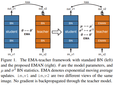
EMA teacher

• Both the student and the teacher use standard BN during training.

• The teacher parameters \(\theta'\) are updated by exponential moving average from the student parameters \(\theta\), \(\theta':=m\theta'+(1-m)\theta\), where \(m\) is the momentum. SGD for students, but no gradient back propagation through the teacher model.

• BN

  • In training, first compute the mean and the variance of the layer inputs for the current batch. Then every sample in the current batch is normalized using the batch-wise statistics, and then an affine transformation with learnable parameters \(\gamma,\beta\) is applied \[ \hat{x}=BN(x)=\gamma \frac{x-\mu_{\mathcal{B}}}{\sqrt{\sigma_{\mathcal{B}}^2}+\epsilon}+\beta, \] where $$ is a small constant for numerical stability.

  • In inference, though the population statistics should be used instead, but since the additional stage, in many implementations, a more practical way is collecting the proxy statistics \(\mu,\sigma^2\) by EMA during training \[ \mu:=\alpha\mu+(1-\alpha)\mu_{\mathcal{B}},\\ \sigma^2:=\alpha\sigma^2+(1-\alpha)\sigma_{\mathcal{B}}^2,\\ \] then the BN at inference becomes \(\hat{x}=BN(x)=\gamma \frac{x-\mu}{\sqrt{\sigma^2}+\epsilon}+\beta,\)

• When the teacher is updated by EMA, the standard BN is not well aligned with the model parameters

  • The teacher is used to generate pseudo GY to guide the learning of the student, the batch-wise BN will make generated labels be cross-sample dependent.
  • Possible mismatch between the model parameters \(\theta'\) and batch-wise BN statistics in the teacher model since the non-alignment of iterations.==> lead to non-smoothness in the parameter space.

EMAN

• Compared with formula (2) in pervious section, they use EMAN for the teacher during training (student still uses BN ) where \(\hat{x}=EMAN(x)=\gamma \frac{x-\mu'}{\sqrt{\sigma'^2}+\epsilon}+\beta,\) where \(\mu',\sigma'^2\) are also exponentially moving averaged from the student \(\mu,\sigma^2\): \[ \mu':=m\mu'+(1-m)\mu,\\ \sigma'^2:=m\sigma'^2+(1-m)\sigma^2,\\ \]

  • This is a linear transform which is no longer dependent on batch statistics.

• Although the student is still cross-sample dependent, this is a less serious issue than the cross-sample dependency in the teacher.

Paper 45: Recognizing Actions in Videos from Unseen Viewpoints

Why

• CNNs are unable to recognize actions/data that are outside of the training data distribution, also unseen viewpoint.
• PoseNet for 3D coordinates, and CalibNet for a limited extrinsic camera matrix.
• But the 3D pose directly from PoseNet may not be the best feature since scale changes, speed of which the action occurs etc.

Goal

• introduce a new geometric convolutional layer that can learn viewpoint invariant representations. The core is to learn and represent the intrinsic camera matrix \(K\).
• Estimating 3D poses, then explores using different representations of it for recognition.

How

• Learn global 3D pose and 2d multi-view projections of it for classifying unseen viewpoints.

  

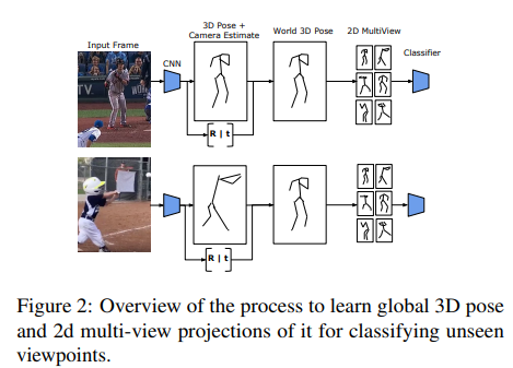
• The 3d world coordinate system is the same for all videos, thus \(R\) is different for each video, depending on the camera viewpoint. \(R\) plays the role of aligning features in different scenes, so that the losses are minimized.

• To enforce the similarity of the 3D representations from the same action and the dissimilarity of 2D view,

  • \(\mathrm{3d\_{loss}}(V,U)=\|F_W(V)-F_W(U)\|_F\),
  • \(cam_reg(c_1,c_2)=\max(-\|c_1,c_2\|_F,\alpha)\)

• The final loss

  

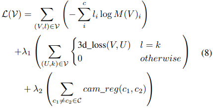
Paper 46: Shot Contrastive Self-Supervised Learning for Scene Boundary Detection

Why

• A shot: a series of frames captured from the same camera over an interrupted period of time. A scene: a series of shots depicting a semantically cohesive part of a story.
• Scenes are more difficult to be localized.
• Previous relatively simple data augmentation used by SSL cannot encode the complex temporal scene-structure.
• Scene detection: define the locations in videos where different scenes begin and end.

Goal

• Find scene boundaries. Propose ShotCoL to Learn a shot representation that maximizes the similarity between nearby shots compared to randomly selected shots, and then use the shot representation to detect scene boundary.
• Use the priors: nearby shots tend to have the same set of actors enacting a semantically cohesive story-arch, and therefore are more similar to each other compared with other randomly selected shots.==>consider nearby shots as augmented versions of each other .
• Specifically, given a shot (both the images and audios), they try to: (a) maximize its similarity with its most similar neighboring shot, and (b) minimize its similarity with a set of randomly selected shots.

How

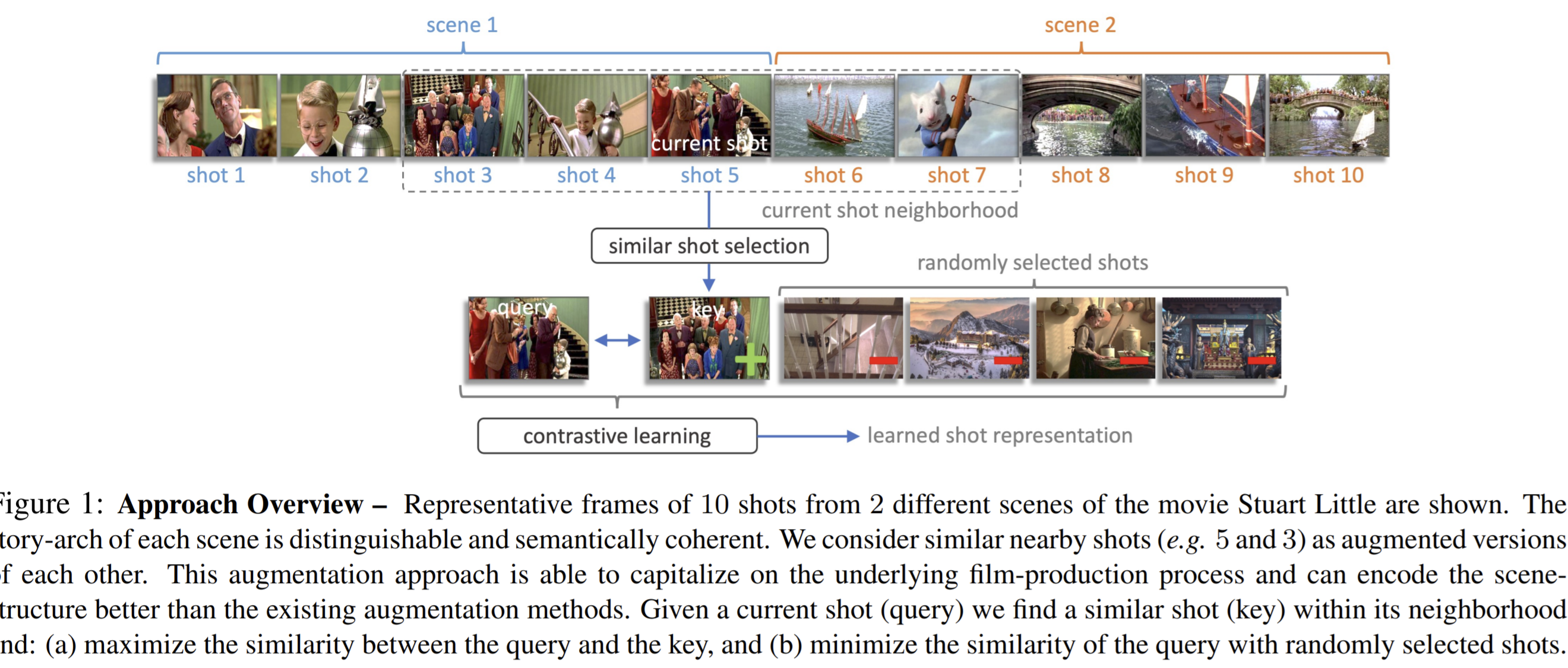
Shot-level representation learning

• Given a full-length input video, use standard shot detection techniques to divide it into its constituent set of shots.
• Comprises of encoder network and momentum contrastive learning to contrast the similarity of the embedded shots.
• Shot encoder network
  • The intra-shot frame dynamics is not as important since scene boundaries depend on inter-shot relationships.
    • Sample \(k\) frames uniformly from each shot, and then reshape the 4D tensor to 3D by combining \(c\) channels and \(k\) frames.
    • Advantages: the usage of standard networks and resource efficiency.
  • Audio modality: use a Wavegram-Longmel CNN which incorporates a 14-layer CNN similar in architecture to the VGG network.
• Shot contrastive learning
  • Pretext: given a query shot, first find the positive key as its most similar shot within a neighborhood around the query, and then maximizes the similarity between the query and the positive key, and minimize the similarity of the query with a set of randomly selected shots.
  • The positive key is the most similar shot compared with the query one in embedded space (after query encoder).
  • The contrastive loss is InfoNCE.
  • Momentum contrast: save the embedded keys in a fixed-sized queue as negative keys, and follow FIFO. And a momentum update scheme is used for the key encoder. \(\theta_k \leftarrow\alpha\theta_k+(1-\alpha)\theta_q\).

Supervised learning

• Formulate the problem of scene boundary detection as a binary classification problem of determining if a shot boundary is also a scene boundary or not.
• For each shot boundary, consider its \(2N\) neighboring shots as a data-point to perform scene boundary detection.
• Use MLP as the classifier of boundary, and take the features extracted from trained shot-level contrastive learning as the input.
• While inference, directly use the features of audio and visual from shot encoder, and the trained MLP.