Paper 1: Vincent et al (2008) Stacked Denoising Autoencoders: Learning Useful Representations in a Deep Network with a Local Denoising Criterion. JMLR 2008
Analysis of SSL methods
- Paper 2: Kolesnikov, Zhai and Beyer (2019) Revisiting Self-Supervised Visual Representation Learning. CVPR 2019
- Paper 3: Zhai et al (2019) A Large-scale Study of Representation Learning with the Visual Task Adaptation Benchmark (A GLUE-like benchmark for images) ArXiv 2019
- Paper 4: Asano et al (2019) A critical analysis of self-supervision, or what we can learn from a single image ICLR 2020
Contrastive methods
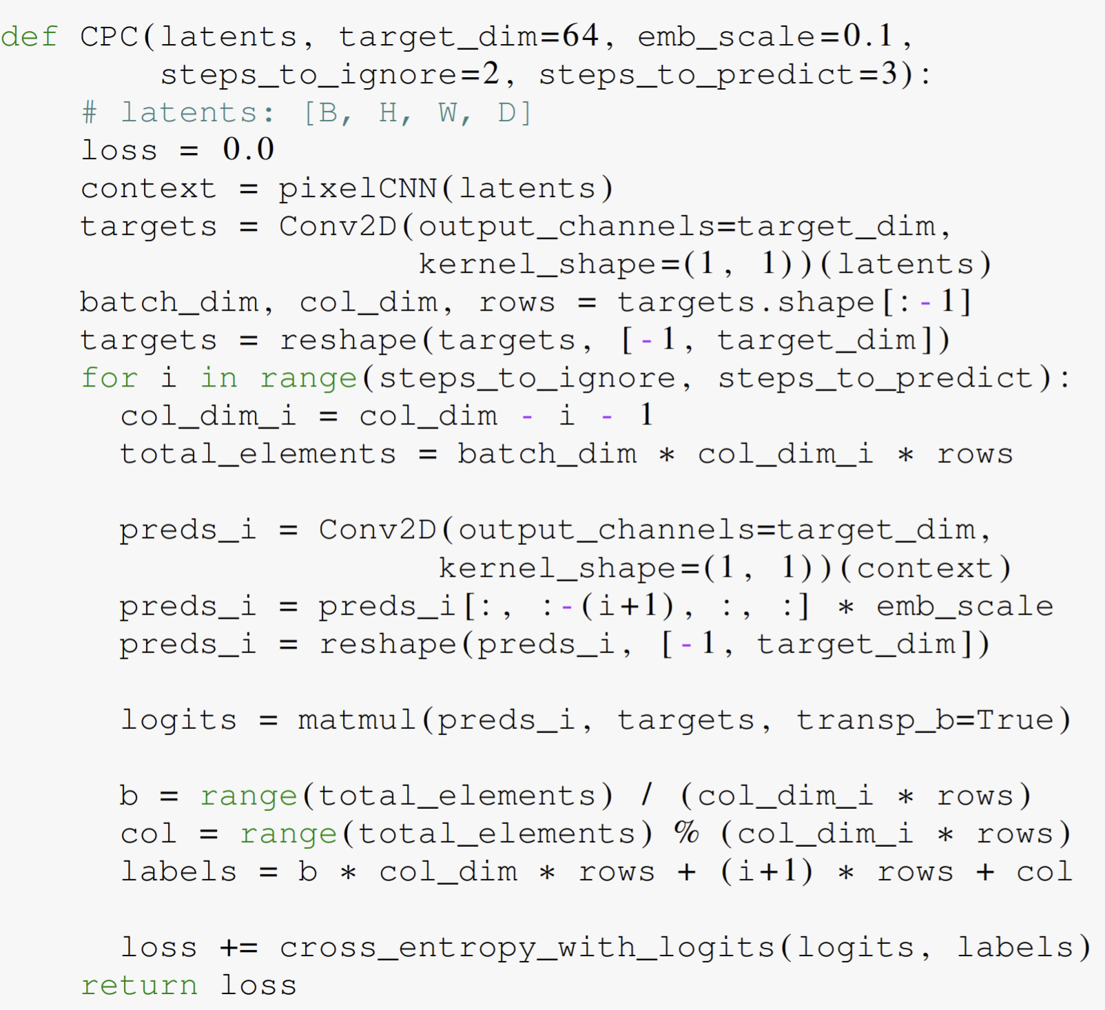
Paper 5: van den Oord et al. (2018) Representation Learning with Contrastive Predictive Coding (CPC), ArXiv 2018
Paper 6: Hjelm et al. (2019) Learning deep representations by mutual information estimation and maximization (DIM) ICLR 2019
Paper 7: Tian et al. (2019) Contrastive Multiview Coding (CMC) ArXiv 2019
Paper 8: Hénaff et al. (2019) Data-Efficient Image Recognition with Contrastive Predictive Coding (CPC v2: Improved CPC evaluated on limited labelled data) ArXiv 2019
Paper 9: He et al (2020) Momentum Contrast for Unsupervised Visual Representation Learning (MoCo, see also MoCo v2). CVPR 2020
Paper 10: Chen T et al (2020) A Simple Framework for Contrastive Learning of Visual Representations (SimCLR). ICML 2020
Paper 11: Chen T et al (2020) Big Self-Supervised Models are Strong Semi-Supervised Learners (SimCLRv2) ArXiv 2020
Paper 12: Caron et al (2020) Unsupervised Learning of Visual Features by Contrasting Cluster Assignments (SwAV) ArXiv 2020
Paper 13: Xiao et al (2020) What Should Not Be Contrastive in Contrastive Learning ArXiv 2020
Paper 14: Misra and van der Maaten (2020) Self-Supervised Learning of Pretext-Invariant Representations. CVPR 2020
Generative methods
- Paper 15: Dumoulin et al (2017) Adversarially Learned Inference (ALI) ICLR 2017
- Paper 16: Donahue, Krähenbühl and Darrell Adversarial Feature Learning (BiGAN, concurrent and similar to ALI) ICLR 2017
- Paper 17: Donahue and Simonyan (2019) Large Scale Adversarial Representation Learning (Big BiGAN) ArXiv 2019
- Paper 18: Chen et al (2020) Generative Pretraining from Pixels (iGPT) ICML 2020
BYoL: boostrap your own latents
- Paper 19: Tarvainen and Valpola (2017) Mean teachers are better role models: Weight-averaged consistency targets improve semi-supervised deep learning results. NeurIPS 2017
- Paper 20: Grill et al (2020) Bootstrap Your Own Latent: A New Approach to Self-Supervised Learning (BYoL). ArXiv 2020
- Paper 21: Abe Fetterman, Josh Albrecht, (2020) Understanding self-supervised and contrastive learning with "Bootstrap Your Own Latent" (BYOL) Blog post
- Paper 22: Schwarzer and Anand et al. (2020) Data-Efficient Reinforcement Learning with Momentum Predictive Representations. ArXiv 2020
self-distillation methods
- Paper 23: Furlanello et al (2017) Born Again Neural Networks. NeurIPS 2017
- Paper 24: Yang et al. (2019) Training Deep Neural Networks in Generations: A More Tolerant Teacher Educates Better Students. AAAI 2019
- Paper 25: Ahn et al (2019) Variational information distillation for knowledge transfer. CVPR 2019
- Paper 26: Zhang et al (2019) Be Your Own Teacher: Improve the Performance of Convolutional Neural Networks via Self Distillation ICCV 2019
- Paper 27: Müller et al (2019) When Does Label Smoothing Help? NeurIPS 2019
- Paper 28: Yuan et al. (2020) Revisiting Knowledge Distillation via Label Smoothing Regularization. CVPR 2020
- Paper 29: Zhang and Sabuncu (2020) Self-Distillation as Instance-Specific Label Smoothing ArXiv 2020
- Paper 30: Mobahi et al. (2020) Self-Distillation Amplifies Regularization in Hilbert Space. ArXiv 2020
self-training / pseudo-labeling methods
- Paper 31: Xie et al (2020) Self-training with Noisy Student improves ImageNet classification. CVPR 2020
- Paper 32: Sohn and Berthelot et al. (2020) FixMatch: Simplifying Semi-Supervised Learning with Consistency and Confidence. ArXiv 2020
- Paper 33: Chen et al. (2020) Self-training Avoids Using Spurious Features Under Domain Shift. ArXiv 2020
Iterated learning/emergence of compositional structure
- Paper 34: Ren et al. (2020) Compositional languages emerge in a neural iterated learning model. ICLR 2020
- Paper 35: Guo, S. et al (2019) The emergence of compositional languages for numeric concepts through iterated learning in neural agents. ArXiv 2020
- Paper 36: Cogswell et al. (2020) Emergence of Compositional Language with Deep Generational Transmission ArXiv 2020
- Paper 37: Kharitonov and Baroni (2020) Emergent Language Generalization and Acquisition Speed are not tied to Compositionality ArXiv 2020
NLP
- Paper 38: Peters et al (2018) Deep contextualized word representations (ELMO), NAACL 2018
- Paper 39: Devlin et al (2019) BERT: Pre-training of Deep Bidirectional Transformers for Language Understanding. (BERT) NAACL 2019
- Paper 40: Brown et al (2020) Language Models are Few-Shot Learners (GPT-3, see also GPT-1and 2for more context) ArXiv 2020
- Paper 41: Clark et al (2020) ELECTRA: Pre-training Text Encoders as Discriminators Rather Than Generators ICLR 2020
- Paper 42: He and Gu et al. (2020) REVISITING SELF-TRAINING FOR NEURAL SEQUENCE GENERATION (Unsupervised NMT) ICLR 2020
video/multi-modal data
- Paper 43: Wang and Gupta (2015) Unsupervised Learning of Visual Representations using Videos ICCV 2015
- Paper 44: Misra, Zitnick and Hebert (2016) Shuffle and Learn: Unsupervised Learning using Temporal Order Verification ECCV 2016
- Paper 45: Lu et al (2019) ViLBERT: Pretraining Task-Agnostic Visiolinguistic Representations for Vision-and-Language Tasks, NeurIPS 2019
- Paper 46: Hjelm and Bachman (2020) Representation Learning with Video Deep InfoMax. (VDIM) Arxiv 2020
the role of noise in representation learning
- Paper 47: Bachman, Alsharif and Precup (2014) Learning with Pseudo-Ensembles NeurIPS 2014
- Paper 48: Bojanowski and Joulin (2017 ) Unsupervised Learning by Predicting Noise. ICML 2017
SSL for RL, control and planning
- Paper 49: Pathak et al. (2017) Curiosity-driven Exploration by Self-supervised Prediction (see also a large-scale follow-up) ICML 2017
- Paper 50: Aytar et al. (2018) Playing hard exploration games by watching YouTube (TDC) NeurIPS 2018
- Paper 51: Anand et al. (2019) Unsupervised State Representation Learning in Atari (ST-DIM) NeurIPS 2019
- Paper 52: Sekar and Rybkin et al. (2020) Planning to Explore via Self-Supervised World Models. ICML 2020
- Paper 53: Schwarzer and Anand et al. (2020) Data-Efficient Reinforcement Learning with Momentum Predictive Representations. ArXiv 2020
SSL theory
- Paper 54: Arora et al (2019) A Theoretical Analysis of Contrastive Unsupervised Representation Learning. ICML 2019
- Paper 55: Lee et al (2020) Predicting What You Already Know Helps: Provable Self-Supervised Learning ArXiv 2020
- Paper 56: Tschannen, et al (2019) On mutual information maximization for representation learning. ArXiv 2019.
Unsupervised domain adaption
- Paper 57: Shu et al (2018) A DIRT-T APPROACH TO UNSUPERVISED DOMAIN ADAPTATION. ICLR 2018
- Paper 58: Wilson and Cook (2019) A Survey of Unsupervised Deep Domain Adaptation. ACM Transactions on Intelligent Systems and Technology 2020.
- Paper 59: Mao et al. (2019) Virtual Mixup Training for Unsupervised Domain Adaptation. CVPR 2019
- Paper 60: Vu et al. (2018) ADVENT: Adversarial Entropy Minimization for Domain Adaptation in Semantic Segmentation CVPR 2019
Scaling
- Paper 61: Kaplan et al (2020) Scaling Laws for Neural Language Models. ArXiv 2020
Paper 1: Stacked Denoising Autoencoders: Learning Useful Representations in a Deep Network with a Local Denoising Criterion
Codes:
Previous
- What works much better is to initially use a local unsupervised criterion to (pre)train each layer in turn, with the goal of learning to produce a useful higher-level representation from the lower-level representation output by the previous layer.
- Initializing a deep network by stacking autoencoders yields almost as good a classification performance as when stacking RBMs. But why is it almost as good?
- looking for unsupervised learning principles likely to lead to the learning of feature detectors that detect important structure in the input patterns.
Traditional classifiers training with noisy inputs
- Training with noise is equivalent to applying generalized Tikhonov regularization (Bishop, 1995), which means L2 weight decay penalty but on linear regression with additive noise. For non-linear case, the regularization is more complex. Authors of this paper even show that different result when using DAEmon and when using regular autoencoders with a L2 weight decay.
Pseudo-Likelihood and Dependency Networks
- Pseudo-likelihood , dependency network paradigms etc.
Ideas
stacking layers of denoising autoencoders which are trained locally to denoise corrupted versions of their inputs. Find that denoising autoencoders are able to learn Gabor-like edge detectors from natural image patches and larger stroke detectors from digit images. our results clearly establish the value of using a denoising criterion as an unsupervised objective to guide the learning of useful higher level representations.
Reasoning: what makes good representations
- A good representation is those that retain a significant amount of information about the input, can be expressed in information-theoretic terms as maximizing the mutual information
- Mutual information can be decomposed into an entropy and a conditional entropy term in two different ways
- ICA:


- consider a parameterized distribution $p(X|Y;') $ that parameterized by \(\mathrm{\theta}'\), then
 leads to maximizing a lower bound on
 and thus on the mutual information.
 - ICA is when \(Y=f_\theta(X)\).
- As \(q(X)\) is unknown, but with samples, the empirical average over the training samples can be used instead as an unbiased estimate (i.e., replacing \(\mathbb{E}_{q(X)}\) by $_{q^0(X)} $:

- consider a parameterized distribution $p(X|Y;') $ that parameterized by \(\mathrm{\theta}'\), then
- ICA:
- The equation above corresponds to the reconstruction error criterion used to train autoencoders
 :
:  To choose \(p(\mathrm{x|z}),L(\mathrm{x|z})\)
- For real-valued $ $ squared error:
 on \(\sigma^2\), the variance of \(X\). Since gaussian, not to use a squashing nonlinearity in the decoder.
 - Binary $ $: finally become cross-entropy loss, which can be used when $ $ is not strictly binary but rather $^d $
- For real-valued $ $ squared error:
- training an autoencoder to minimize reconstruction error amounts to maximizing a lower bound on the mutual information between input X and learnt representation Y
- Merely Retaining Information is Not Enough
- non-zero reconstruction error to separate useful information from noise: traditional AE uses bottleneck to produce an under-complete representation where \(d'<d\), and result in a lossy compressed representation of \(X\). When using affine encoder and decoder without any nonlinearity an a squared error loss, the AE performs PCA actually. But not in cross-entropy loss.
- using over-complete (i.e., higher dimensional than the input) but sparse representations is popular now, which is a special case of imposing on \(Y\) different constraints than that of a lower dimensionality. A sparse over-complete representations can be viewed as an alternative “compressed” representation.
How?
DAE: denoising autoencoder
Procedures
- first denoising: corrupt the initial input $ $ into \(\tilde{\mathrm{x}}\) by a stochastic mapping. This will lead to force the learning of a mapping that extracts features useful for denoising.
- Then map \(\tilde{\mathrm{x}}\) to \(\mathrm{y}\). And reonstruct \(\mathrm{z}\) to be close to the $ $ but a function of \(\mathrm{y}\).
Geometric Interpretation
- Thus stochastic operator \(p(X|\tilde{X})\) learns a map that tends to go from lower probability points \(\tilde{X}\) to nearby high probability points \(X\), on or near the manifold.
- Successful denoising implies that the operator maps even far away points to a small region close to the manifold
- Think of \(Y=f(X)\) as a representation of \(X\) which is well suited to capture the main variations in the data, that is, those along the manifold.
Types of corruption considered
- additive: natural
- masking noise: natural for input domains which are interpretable as binary or near binary such as black an white images or the representation produced at the hidden layer after a signoid squashing function
- salt and pepper noise: same as masking noise, only earse a changing subsets of the inputs components while leaving others untouched
Emphasize corrupted dimensions
only put an emphasis on the corrupted dimensions. Like use \(\alpha\) for the Reconstruction error on corrupted components and \(\beta\) for untouched components
Sqaured loss

Cross-entropy loss

If \(\alpha=1, \beta=0\), then this is full emphasis that only consider the error on the prediction of corrupted elements
Stacking DAE for deep architecture
Experiments
Single DAE
- feature detectors from natural image patches
- The under-complete autoencoder appears to learn rather uninteresting local blob detectors. Filters obtained in the overcomplete case have no recognizable structure, looking entirely random
- training with sufficiently large noise yields a qualitatively very different outcome than training with a weight decay regularization and this proves that the two are not equivalent for a non-linear autoencoder.
- Salt-and-pepper noise yielded Gabor-like edge detectors, whereas masking noise yielded a mixture of edge detectors and grating filters. They all yield some potentially useful edge detectors.
- feature detectors from handwrite digits
- With increased noise levels, a much larger proportion of interesting (visibly non random and with a clear structure) feature detectors are learnt. These include local oriented stroke detectors and detectors of digit parts such as loops.
- But denoising a more corrupted input requires detecting bigger, less local structures.
- feature detectors from natural image patches
Stacked DAE (SDAE): compare with SAE and DBN.
- Classification problem and experimental methodology: As increasing the noise level, denoising training forces the filters to differentiate more, and capture more distinctive features. Higher noise levels tend to induce less local filters, as expected.
- Compared with other strategies: denoising pretraining with a non-zero noise level is a better strategy than pretraining with regular autoencoders
- Influence of Number of Layers, Hidden Units per Layer, and Noise Level
- Depth: denoising pretraining being better than autoencoder pretraining being better than no pretraining. The advantage appears to increase with the number of layers and with the number of hidden units
- noise levels: SDAE appears to perform better than SAE (0 noise) for a rather wide range of noise levels, regardless of the number of hidden layers.
Denoising pretraining v.s. training with noisy input
- Note: SDAE uses a denoising criterion to learn good initial feature extractors at each layer that will be used as initialization for a noiseless supervised training; which is different from training with noisy inputs that amounts to training with a virtually expanded data set.
- Denoising pretraining with SDAE, for a large range of noise levels, yields significantly improved performance, whereas training with noisy inputs sometimes degrades the performance, and sometimes improves it slightly but is clearly less beneficial than SDAE.
Variations on the DAE, alternate corruption types and emphasizing
- An emphasized SDAE with salt-and-pepper noise appears to be the winning SDAE variant.
- A judicious choice of noise type and added emphasis may often buy us a better performance.
Are Features Learnt in an Unsupervised Fashion by SDAE Useful for SVMs?
- SVM performance can benefit significantly from using the higher level representation learnt by SDAE
- linear SVMs can benefit from having the original input processed non-linearly
Generating Samples from Stacked Denoising Autoencoder Networks
- Top-Down Generation of a Visible Sample Given a Top-Layer Representation: it is thus possible to generate samples at one layer from the representation of the layer above in the exact same way as in a DBN.
- Bottom-up (infer representation of the top layer based on representation on the bottom layer) is similar as approximate inference of a factorial Bernoulli top-layer distribution given the low level input. The top-layer representation is to be understood as the parameters (the mean) of a factorial Bernoulli distribution for the actual binary units.
- SDAE and DBN are able to resynthesize a variety of similarly good quality digits, whereas the SAE trained model regenerates patterns with much visible degradation in quality, this also prove that evidence of the qualitative difference resulting from optimizing a denoising criterion instead of mere reconstruction criterion.
- Contrary to SAE, the regenerated patterns from SDAE or DBN look like they could be samples from the same unknown input distribution that yielded the training set.
Paper 2: Revisiting Self-Supervised Visual Representation Learning
https://github.com/google/revisiting-self-supervised
Previous
- Compared with pretext task, the choice of CNN has not received equal attention
- patch-based self-supervised visual representation learning methods: predicting the relative location of image patches; “jigsaw puzzle” created from the full image etc.
- image-level classification tasks: randomly rotate an image by one of four possible angles and let the model predict that rotation; use clustering of the images
- tasks with dense spatial outputs: image inpainting, image colorization, its improved variant split-brain and motion segmentation prediction.
- equivariance relation to match the sum of multiple tiled representations to a single scaled representation; predict future patches in via autoregressive predictive coding.
- many works have tried to combine multiple pretext tasks in one way or another
What?
- Standard architecture design recipes do not necessarily translate from the fully-supervised to the self-supervised setting. Architecture choices which negligibly affect performance in the fully labeled setting, may significantly affect performance in the self-supervised setting.
- The quality of learned representations in CNN architectures with skip-connections does not degrade towards the end of the model.
- Increasing the number of filters in a CNN model and, consequently, the size of the representation significantly and consistently increases the quality of the learned visual representations.
- The evaluation procedure, where a linear model is trained on a fixed visual representation using stochastic gradient descent, is sensitive to the learning rate schedule and may take many epochs to converge.
How
- revisit a prominent subset of the previously proposed pretext tasks and perform a large-scale empirical study using various architectures as base models.
- The CNN candidates
- ResNet:
- RevNet: stronger invertibility guarantees while being structurally similar to ResNets. Set it to have the same depth and number of channels as the original Resnet50 model.
- VGG: no skip, has BN
- The pretext tasks candidates
- Rotation: 0,90,180,270
- Exemplar: heavy random data augmentation such as translation, scaling, rotation, and contrast and color shifts
- Jigsaw: recover relative spatial position of 9 randomly sampled image patches after a random permutation of these patches. They extract representations by averaging the representations of nine uniformly sampled, colorful, and normalized patches of an image.
- Relative patch location: 8 possible relative spatial relations between two patches need to be predicted. use the same patch prepossessing as in the Jigsaw model and also extract final image representations by averaging representations of 9 cropped patches.
- Dataset candidates
- ImageNet
- Places205
- Evaluation protocol
- measures representation quality as the accuracy of a linear regression model trained and evaluated on the ImageNet dataset
- the pre-logits of the trained self-supervised networks as representation.
Experiments
similar models often result in visual representations that have significantly different performance. Importantly, neither is the ranking of architectures consistent across different methods, nor is the ranking of methods consistent across architectures
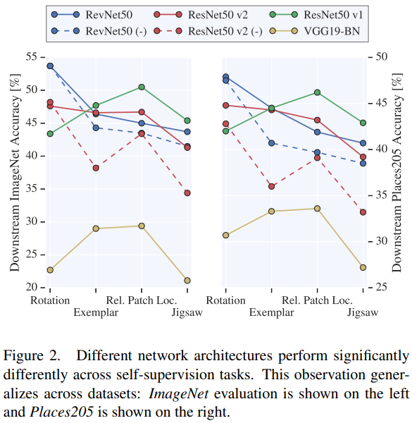
increasing the number of channels in CNN models improves performance of self-supervised models.
ranking of models evaluated on Places205 is consistent with that of models evaluated on ImageNet, indicating that our findings generalize to new datasets.
self-supervised learning architecture choice matters as much as choice of a pretext task
MLP provides only marginal improvement over the linear evaluation and the relative performance of various settings is mostly unchanged. We thus conclude that the linear model is adequate for evaluation purposes.
Better performance on the pretext task does not always translate to better representations. For residual architectures, the pre-logits are always best.
Skip-connections prevent degradation of representation quality towards the end of CNNs. We hypothesize that this is a result of ResNet’s residual units being invertible under some conditions. RevNet, boosts performance by more than 5 % on the Rotation task, albeit it does not result in improvements across other tasks.
Model width and representation size strongly influence the representation quality: disentangle the network width from the representation size by adding an additional linear layer to control the size of the pre-logits layer. self-supervised learning techniques are likely to benefit from using CNNs with increased number of channels across wide range of scenarios.
SGD optimization hyperparameters play an important role and need to be reported. very long training (≈ 500 epochs) results in higher accuracy. They decay lr at 480 epochs.
Paper 3: Zhai et al (2019) A Large-scale Study of Representation Learning with the Visual Task Adaptation Benchmark (A GLUE-like benchmark for images)
https://github.com/google-research/task_adaptation
Previous
- the absence of a unified evaluation for general visual representations hinders progress. Each sub-domain has its own evaluation protocol, and the lack of a common benchmark impedes progress.
- Popular protocols are often too constrained (linear classification), limited in diversity (ImageNet, CIFAR, Pascal-VOC), or only weakly related to representation quality (ELBO, reconstruction error)
What?
- present the Visual Task Adaptation Benchmark (VTAB), which defines good representations as those that adapt to diverse, unseen tasks with few examples. (i) minimal constraints to encourage creativity, (ii) a focus on practical considerations, and (iii) make it challenging.
- Conduct a large-scale study of many popular publicly-available representation learning algorithms on VTAB.
- They found:
- Supervised ImageNet pretraining yields excellent representations for natural image classification tasks
- Self-supervised is less effective than supervised learning overall, but surprisingly, can improve structured understanding
- Combining supervision and self-supervision is effective, and to a large extent, self-supervision can replace, or compliment labels.
- Discriminative representations appear more effective than those trained as part of a generative model, with the exception of adversarially trained encoders.
- GANs perform relatively better on data similar to their pre-training source (here, ImageNet), but worse on other tasks.
- Evaluation using a linear classifier leads to poorer transfer and different conclusions.
How?
- To design, must ensure that the algorithms are not pre-exposed to specific evaluation samples.
- VTAB benchmark
- practical benchmark
- Define task distribution as Tasks that a human can solve, from visual input alone.”
- For each evaluation sample a new task.
- mitigating meta-overfitting : treat the evaluation tasks unseen, and thus algorithms use pretraining must not pre-train on any of the evaluation tasks.
- Unified implementation: algorithms must have no prior knowledge of the downstream tasks, and hyperparameter searches need to work well across the benchmark.
- All tasks are classification in this paper, such as the detection task is mapped to the classification of the \((x,y,z)\) coordinates. The diverse set of visual features are learnt from object identification, scene classification, pathology detection, counting, localization and 3D geometry.
- Tasks
- NATURAL: classical vision problems, group includes Caltech101, CIFAR100, DTD, Flowers102, Pets, Sun397, and SVHN
- SPECIALIZED: images are captured through specialist equipment, and human can recognize the structures. One is remote sensing, the other is medical
- STRUCTURED: assesses comprehension of the structure of a scene, for example, object counting, or 3D depth prediction.
- pretraining on pretext tasks and then fine tune
- practical benchmark
- The methods are divided into five groups: Generative, training from-scratch, all methods using 10% labels (Semi Supervised), and all methods using 100% labels (Supervised),
Experiments
- Upstream, control the data and architecture (pretrained on ImageNet). They find bigger architectures perform better on VTAB, and use resnet or resnet-similar nets for all models as the encoder.
- Downstream, run VTAB in two modes: the light weight mode sweepstakes 2 initial learning rates and 2 learning rate schedules but fix other parameters while the heavy weights perform a large random search over learning rate, schedule, optimizers, batch size, train preprocessing functions, evaluation preprocessing and weight decay. The main study is done in lightweight.
- Evaluate with top-1 accuracy. To aggregate scores across tasks, take the mean accuracy.
- Lightweight
- Generative models perform worst, GANs fit more strongly to ImageNet’s domain (natural images), than self-supervised alternatives.
- All self-supervised representations outperform from-scratch training. Methods applied to the entire image outperform patch-based method, and these tasks require sensitivity to local textures. self supervised is worst than supervised on natural tasks, similar on specialized tasks and slightly better than structured tasks.
- Supervised models perform the best. additional self-supervision even improves on top of 100% labelled ImageNet, particularly on STRUCTURED tasks
- Heavyweight
- across all task groups, pre-trained representations are better than a tuned from-scratch model.
- a combination supervision and self-supervision (SUP-EXEMPLAR-100%) getting the best performance.
- Frozen feature extractors
- linear evaluation significantly lowers performance, even when downstream data is limited to 1000 examples. Linear transfer would not by used in practice unless infrastructural constraints required it. These self-supervised methods extract useful representations, just without linear separability. Linear evaluation results are sensitive to additional factors that we do not vary, such as ResNet version or pre-training regularization parameters.
- Vision benchmarks
- The methods ranked according to VTAB are more likely to transfer to new tasks, than those ranked according to the Visual Decathlon
- VTAB is more flexible than Facebook AI SSL challenge, such as the diversity of domain, the evaluation form.
- Meta-dataset: designed for few-shot learning rather than 1000 examples which may entail different solutions.
- Some details
- while training from scratch , inception crop, horizontal flip preprocessing, 1e-3 in weight decay, 0.1~1 lr in SGD mostly give good results.
- While doing SSL by ImageNet and then finetuning, Inception crop, non-horizontal flip give good results.
Discussion
- how effective are supervised ImageNet representations? ImageNet labels are indeed effective for natural tasks.
- how do representations trained via generative and discriminative models compare? The generative losses seem less promising as means towards learning how to represent data. BigBiGAN is notable.
- To what extent can self-supervision replace labels?
- self-supervision can almost (but not quite) replace 90% of ImageNet labels; the gap between pre-training on 10% labels with self-supervison, and 100% labels, is small
- self-supervision adds value on top of ImageNet labels on the same data.
- simply adding more data on the SPECIALIZED and STRUCTURED tasks is better than the pre-training strategies we evaluated
- Varying other factors to improve VTAB is valuable future research. The only approach that is out-of-bounds is to condition the algorithm explicitly on the VTAB tasks
Paper 4: A critical analysis of self-supervision, or what we can learn from a single image
https://github.com/yukimasano/linear-probes
Previous
- For a given model complexity, pre-training by using an off-the-shelf annotated image datasets such as ImageNet remains much more efficient.
- Methods often modify information in the images and require the network to recover them. However, features are learned on modified images which potentially harms the generalization to unmodified ones.
- Learning from a single sample
- Object tracking: max margin correlation filters learn robust tracking templates from a single sample of the patch.
- learn and interpolate multi-scale textures with a GAN framework
- semi-parametric exemplar SVM model
- we do not use a large collection of negative images to train our model. Instead we restrict ourselves to a single or a few images with a systematic augmentation strategy.
- Classical learned and hand-crafted low-level feature extractors: insufficient to clarify the power and limitation of self-supervision in deep networks.
What
- Aim to investigate the effectiveness of current self-supervised approaches by characterizing how much information they can extract from a given dataset of images. Then try to answer whether a large dataset is beneficial to unsupervised learning, especially for learning early convolutional features
- Three different and representative methods, BiGAN, RotNet and DeepCluster, can learn the first few layers of a convolutional network from a single image as well as using millions of images and manual labels, provided that strong data augmentation is used.
- For deeper layers the gap with manual supervision cannot be closed even if millions of unlabelled images are used for training.
- Conclusion
- the weights of the early layers of deep networks contain limited information about the statistics of natural images
- such low-level statistics can be learned through self-supervision just as well as through strong supervision, and that
- the low-level statistics can be captured via synthetic transformations instead of using a large image dataset. (training these layers with self-supervision and a single image already achieves as much as two thirds of the performance that can be achieved by using a million different images.)
How
- Data: use DAA augmentation to replace some source images.
- Augmentations: involving cropping, scaling, rotation, contrast changes, and adding noise. Augmentation can be seen as imposing a prior on how we expect the manifold of natural images to look like
- limit the size of cropped patch: the smallest size of the crops is limited to be at least βWH and at most the whole image. Additionally, changes to the aspect ratio are limited by γ. In practice we use β = 10e−3 and γ = 3/4 .
- before cropping, rotate in \((-35,35)\) degrees. And also flip images in 50% possibility
- linear transformation in RGB space, color jitter with additive brightness, contrast and saturation
- Real samples: give some drawn samples which are not real captured but has plenty of textures and in small size, and a real picture in large size but with large areas no objects.
- Augmentations: involving cropping, scaling, rotation, contrast changes, and adding noise. Augmentation can be seen as imposing a prior on how we expect the manifold of natural images to look like
- Representation learning methods
- BiGAN with leaky ReLU nonlinearities in discriminators
- Rotation: do it on horizontal flips and non-scaled random crops to 224 × 224
- clustering:
Experiments
- ImageNet and CIFAR-10/100 using linear probes
- Base encoder: AlexNet. They insert the probes right after the ReLU layer in each block
- Learning lasts for 36 epochs and the learning rate schedule starts from 0.01 and is divided by five at epochs 5, 15 and 25
- extracting 10 crops for each validation image (four at the corners and one at the center along with their horizontal flips) and averaging the prediction scores before the accuracy is computed.
- Effect of augmentations: Random rescaling adds at least ten points at every depth (see Table 1 (f,h,i)) and is the most important single augmentation. Color jittering and rotation slightly improve the performance of all probes by 1- 2% points
- Benchmark evaluation
- Mono is enough: Mono means train with one source image and its augmented images.
- Image contents:
- RotNet cannot extract photographic bias from a single image. the method can extract rotation from low level image features such as patches which is at first counter intuitive=> lighting and shadows even in small patches can indeed give important cues on the up direction which can be learned even from a single (real) image.
- the augmentations can even compensate for large untextured areas and the exact choice of image is not critical. A trivial image without any image gradient (e.g. picture of a white wall) would not provide enough signal for any method.
- More than one image
- for conv1 and conv2, a single image is enough
- In deeper layers, DeepCluster seems to require large amounts of source images to yield the reported results as the deka- and kilo- variants start improving over the single image case
- Generalization
- GAN trained on the smaller Image B outperforms all other methods including the fully-supervised trained one for the first convolutional layer
- our method allows learning very generalizable early features that are not domain dependent.
- the neural network is only extracting patterns and not semantic information because we do not find any neurons particularly specialized to certain objects even in higher levels as for example dog faces or similar which can be fund in supervised networks
Paper 5: Representation Learning with Contrastive Predictive Coding (CPC), ArXiv 2018
Previous
- It is not always clear what the ideal representation is and if it is possible that one can learn such a representation without additional supervision or specialization to a particular data modality.
- One of the most common strategies for unsupervised learning has been to predict future, missing or contextual information
- Recently in unsupervised learning some learn word representations by predicting neighboring words.
- For images, predicting color from grey-scale or the relative position of image patches
- predicting high-dimensional data
- unimodal losses such as mean-squared error and cross-entropy are not very useful
- powerful conditional generative models which need to reconstruct every detail in the data are usually required.
What
- Main contributions
- Compress features into a latent embedding space in which conditional predictions are easier to model.
- predict the future in latent space by autoregressive models
- Use NCE loss
- Intuition
- learn the representations that encode the underlying shared information between parts of the signal
- meanwhile discard low-level information and noise that is more local.
How
- use a NCE which induces the latent space to capture information that is maximally useful to predict future samples
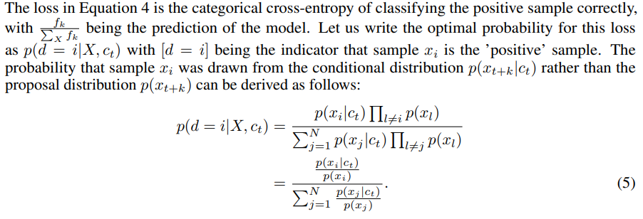
- Model a density ratio which preserves the mutual information between \(x_{t+k},c_t\) as \(f_k(x_{t+k},c_t)\propto \frac{p(x_{t+k}|c_t)}{p(x_{t+k})}\), they choose \(f_k(x_{t+k},c_t)=\exp(z_{t+k}^TW_kc_t)\), the log-bilinear model.
Experiments
For every domain we train CPC models and probe what the representations contain with either a linear classification task or qualitative evaluations.
- Audio
- use a 100-hour subset of the publicly available LibriSpeech dataset
- use a GRU for the autoregressive part of the model
- We found that not all the information encoded is linearly accessible.
- CPCs capture both speaker identity and speech contents
- Vision
- Use ImageNet and ResNet v2 101, no BN. use the outputs from the third residual block, and spatially mean-pool to get a single 1024-d vector per 64x64 patch. This results in a 7x7x1024 tensor. Next, we use a PixelCNN-style autoregressive model to make predictions about the latent activations in following rows top-to-bottom.
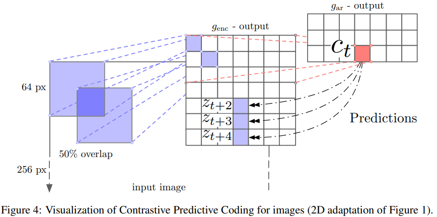
- CPCs improve upon state-of-the-art by 9% absolute in top-1 accuracy, and 4% absolute in top-5 accuracy.
- Natural language
- a linear mapping is constructed between word2vec and the word embeddings learned by the model. A L2 regularization weight was chosen via cross-validation (therefore nested cross-validation for the first 4 datasets)
- found that more advanced sentence encoders did not significantly improve the results, which may be due to the simplicity of the transfer tasks, and the fact that bag-of-words models usually perform well on many NLP tasks.
- The performance of our method is very similar to the skip-thought vector model, with the advantage that it does not require a powerful LSTM as word-level decoder, therefore much faster to train
- Reinforcement learning
- take the standard batched A2C agent as base model and add CPC as an auxiliary loss
- The unroll length for the A2C is 100 steps and we predict up to 30 steps in the future to derive the contrastive loss
- 4 out of the 5 games performance of the agent improves significantly with the contrastive loss after training on 1 billion frames.
Paper 6: Learning deep representations by mutual information estimation and maximization (DIM Deep InfoMax ) ICLR 2019
https://github.com/rdevon/DIM
Previous
- in typical settings, models with reconstruction-type objectives provide some guarantees on the amount of information encoded in their intermediate representations.
- MI estimation
- MINE: strongly consistent, can be used to learn better implicit bidirectional generative models
- DIM: follow MINE, but they find the generator is unnecessary. And no necessary for the exact KL-divergence, alternatively the JSD is more stable and provides better results.
- CPC and DIM
- CPC: make predictions about specific local features in the “future” of each summary feature. This equates to ordered autoregression over the local features, and requires training separate estimators for each temporal offset at which one would like to predict the future.
- DIM uses a single summary feature that is a function of all local features, and this “global” feature predicts all local features simultaneously in a single step using a single estimator.
What
- structure matters: maximizing the average MI between the representation and local regions of the input can improve performance while maximizing MI between the complete input and the encoder output not always do this.
- JSD helps MI estimation. JSD and DVD all maximize the expected log-ratio of the joint over the product of marginals.
How
Mutual information estimation and maximization
Basic MI maximization framework
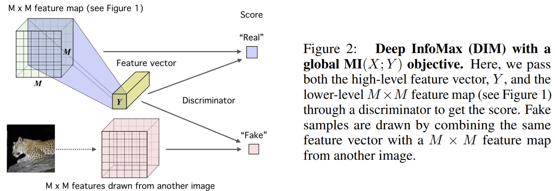
share layers between encoder and mutual information
The different losses of DIM with different estimator
- With non-KL divergences such as JSD:

- With NCE,

- For DIM, a key difference between the DV, JSD, and infoNCE formulations is whether an expectation over \(\mathrm{\mathbb{P/ \tilde{P}}}\) appears inside or outside of a \(\log\). DIM sets the noise distribution to the product of marginals over \(X/Y\) , and the data distribution to the true joint.
- With non-KL divergences such as JSD:
infoNCE often outperforms JSD on downstream tasks, though this effect diminishes with more challenging data and also requires more negative samples compare with the JSD version.
DIM with the JSD loss is insensitive to the number of negative samples, and in fact outperforms infoNCE as the number of negative samples becomes smaller.
Local mutual information maximization
- To obtain a representation more suitable for classification, one can maximize the average MI between the high-level representation and local patches of the image.
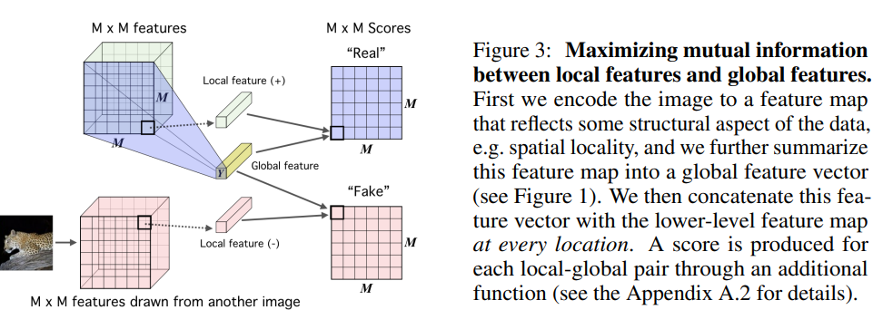
- summarize this local feature map into a global feature
- then the MI estimator on global/local pairs, maximizing the average estimated MI:

Matching representation to a prior distribution
A good representation can be compact, independent, disentangled or independently controllable.
DIM imposes statistical constraints onto learned representations by implicitly training the encoder so that the push-forward distribution, \(\mathrm{\mathbb{U}}_{\psi,\mathrm{\mathbb{P}}}\), matches a prior, \(\mathrm{\mathbb{V}}\).
This is done by training a discriminator \(D_\phi: \mathcal{Y}\rightarrow \mathrm{\mathbb{R}}\) to estimate the divergence, \(\mathcal{D}(\mathrm{\mathbb{V}}|\mathrm{\mathbb{U}}_{\psi,\mathrm{\mathbb{P}}})\). Then training the encoder to minimize

trains the encoder to match the noise implicitly rather than using a priori noise samples as targets
Complete loss

Experiments
- Datasets: CIFAR10+CIFAR100, Tiny ImageNet, STL-10, CelebA (a face image dataset )
- Compared methods: VAE, \(\beta\)-VAE, adversarial AE, BiGAN, NAT, and CPC.
Evaluate the quality of a representation
- Linear separability has no help in showing the representation has high MI with the class labels when the representation is not disentangled.
- To measure:
- They use MINE to more directly measure the MI between the input the the output of the encoder.
- NDM (neural dependency measure): Then measure the independence of the representation using a discriminator. train a discriminator to estimate the KL-divergence between the original representations (joint distribution of the factors) and the shuffled representations. The higher the KL-divergence, the more dependent the factors. NDM is sensible and empirically consistent.
- The classification
- Linear classification
- Non-linear classification (with a single hidden layer NN)
- Semi-supervised learning: finetuning the encoder by adding a small NN.
- MS-SSIM: decoder trained on the L2 Reconstruction loss.
- MINE: maximized the DV estimator of the KL-divergence
- NDM: using a second discriminator to measure the KL between \(E_\psi(x)\) and a batch-wise shuffled version of \(E_\psi(x)\).
Representation learning comparison across models
- Test DIM(G) the global only, DIM (L) the local only and ablation study.
- Classification:
- DIM(L) outperforms all models. The representations are as good as or better than the raw pixels given the model constraints in this setting
- infoNCE tends to perform best, but differences between infoNCE and JSD diminish with larger datasets
- Overall DIM only slightly outperforms CPC in this setting, which suggests that the strictly ordered autoregression of CPC may be unnecessary for some tasks.
- Extended comparison: For MI, DIM combining local and global DIM objectives had very high scores .
- Adding coordinate information and occlusions
- can be interpreted as context prediction and generalizations of inpainting respectively.
- For occlusion: occluded part of input for global representations, but no occlusion for local representations. Maximizing MI between occluded global features and unoccluded local features aggressively encourages the global features to encode information which is shared across the entire image.
Appendix
- KL (traditional definition of mutual information) and the JSD have an approximately monotonic relationship. Overall, the distributions with the highest mutual information also have the highest JSD.
- We found both infoNCE and the DV-based estimators were sensitive to negative sampling strategies, while the JSD-based estimator was insensitive.
- DIM with a local-only objective, DIM(L), learns a representation with a much more interpretable structure across the image.
- In general, good classification performance is highly dependent on the local term, \(\beta\), while good reconstruction is highly dependent on the global term, \(\alpha\). the local objective is crucial, the global objective plays a stronger role here than with other datasets.
Paper 7: Contrastive Multiview Coding (CMC) ArXiv 2019
http://github.com/HobbitLong/CMC/
Previous
- some bits are in fact better than others.
- In these models, an input \(X\) to the model is transformed into an output \(\hat{X}\), which is supposed to be close to another signal \(Y\) (usually in Euclidean space), which itself is related to \(X\) in some meaningful way. and provides us with nearly infinite amounts of training data.
- The objective functions are usually reconstruction-based loss or contrastive losses.
- CPC learns from the past and the future view simultaneously, while Deep InfoMax takes the past as the input and the future as the output. They both use instance discrimination learns to match two sub-crops of the same image.
- They extend the objective to the case of more than two views and explore a different set of view definitions, architectures and application settings.
What
- Idea: a powerful representation is one that models view-invariant factor. We learn a representation that aims to maximize mutual information between different views of the same scene but is otherwise compact.
- study the setting where the different views are different image channels, such as luminance, chrominance, depth, and optical flow. The fundamental supervisory signal we exploit is the co-occurrence, in natural data, of multiple views of the same scene.
- Goal: learn information shared between multiple sensory channels but that are otherwise compact (i.e. discard channel-specific nuisance factors). we learn a feature embedding such that views of the same scene map to nearby points (measured with Euclidean distance in representation space) while views of different scenes map to far apart points.
- Use CPC as the backbone but remove the recurrent network part.
- We find that the quality of the representation improves as a function of the number of views used for training.
- demonstrate that the contrastive objective is superior to cross-view prediction.
How
Suppose a dataset of \(V_1, V_2\) that consists of a collection of samples \(\{v_1 ^i, v_2 ^i\}_{i=1}^N\), consider $x={v_1 ^i, v_2 ^i} $ as the positive and the \(y=\{v_1 ^i, v_2 ^j\}\) as the negatives, aka the positive are the same picture in different views while the negative are the dissimilar images in different views.
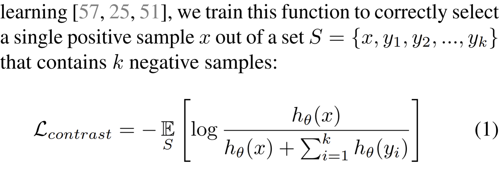 , simply fix one view and enumerate positives and negatives from the other view, then the objective is written as
But directly minimizing the above function is infeasible since \(k\) is pretty large. To approximate,
- Implementing the critic: implement \(h_\theta(\cdot)\) as a neural network. For each view, build a NN as the encoder, then compute the features cosine similarity as score and adjust its dynamic range by a hyper-parameter \(\tau\). The two view loss is then \(\mathcal{L} (V_1,V_2) = \mathcal{L}_{constrast}^{V_1,V_2}+\mathcal{L}_{constrast}^{V_2,V_1}\).
- Connecting to mutual information: minimizing the objective L maximizes the lower bound on the mutual information. But recent works show that the bound can be very weak.
Multi-views
- the full graph formulation is that it can handle missing information (e.g. missing views) in a natural manner.

- The core view is
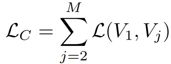
- the full graph formulation is that it can handle missing information (e.g. missing views) in a natural manner.
To estimate, they use memory bank to store latent features for each training sample.
Experiments
- Benchmarks: ImageNet and STL-10.
Benchmarking CMC on ImageNet
- Convert the RGB images to the Lab image color space and split each image into L and ab channels.
- L and ab from the same image are treated as the positive pair, and ab channels from other randomly selected images are treated as a negative pair (for a given L)
- set the temperature τ as 0.07 and use a momentum 0.5 for memory update.
- learning from luminance and chrominance views in two colorspaces, {L, ab} and {Y, DbDr}.
- {Y, DbDr} provides \(0.7\%\) improvement, strengthening data augmentation with RandAugment yields better or comparable results to other SOTA methods.
CMC on videos
- given an image it that is a frame centered at time \(t\), the ventral stream associates it with a neighbouring frame \(i_{t+k}\), while the dorsal stream connects it to optical flow \(f_t\) centered at \(t\).
- extract \(i_t\), \(i_{t+k}\) and \(f_t\) from two modalities as three views of a video.
- Take \((i_t,i_{t+k})\) as the positive, and negative pairs for \(i_t\) is chosen as a random frame from another randomly chosen video;
- Take \((i_t,f_t)\) as the positive, then negative pairs for \(i_t\) are those flow corresponding to a random frame in another randomly chosen video.
- Pretrain the encoder on UCF101 and use two CaffeNets for extracting features from images and optical flows.
- Increasing the number of views of the data from 2 to 3 (using both streams instead of one) provides a boost for UCF-101
Extending CMC to more views
- Consider views: luminance (L channel), chrominance (ab channel), depth, surface normal, and semantic labels.
- the sub-patch based contrastive objective to increase the number of negative pairs
- Does representation quality improve as number of views increases?
- UNet style architecture
- The 2-4 view cases contrast L with ab, and then sequentially add depth and surface normals.
- measured by mean IoU over all classes and pixel accuracy.
- performance steadily improves as new views are added
- Is CMC improving all views?
- train these encoders following the full graph paradigm, where each view is contrasted with all other views.
- evaluate the representation of each view v by predicting the semantic labels from only the representation of v, where v is L, ab, depth or surface normals.
- the full-graph representation provides a good representation learnt for all views.
Predictive Learning vs. Contrastive Learning
- consider three view pairs on the NYU-Depth dataset: (1) L and depth, (2) L and surface normals, and (3) L and segmentation map. For each of them, we train two identical encoders for L, one using contrastive learning and the other with predictive learning.
- evaluate the representation quality by training a linear classifier on top of these encoders on the STL-10 dataset
- For predictive learning, pixel-wise reconstruction losses usually impose an independence assumption on the modeling. While contrastive learning does not assume conditional independence across dimensions of \(v_2\). Also the use of random jittering and cropping between views allows the contrastive learning approach to benefit from spatial co-occurrence (contrasting in space) in addition to contrasting across views.
How does mutual information affect representation quality?
cross-view representation learning is effective because it results in a kind of information minimization, discarding nuisance factors that are not shared between the views.
a good collection of views is one that shares some information but not too much
To test, build two domains: learning representations on images with different colorspaces forming the two views; and learning representations on pairs of patches extracted from an image, separated by varying spatial distance. (use high resolution images to avoid overlapping and cropped patches around boundary.)
using colorspaces with minimal mutual information give the best downstream accuracy
For patches with different offset with each other, views with too little or too much MI perform worse.
the relationship between mutual information and representation quality is meaningful but not direct.
patch-based contrastive loss is computed within each mini-batch and does not require a memory bank, but usually yields suboptimal results compared to NCE-based contrastive loss, according to our experiments
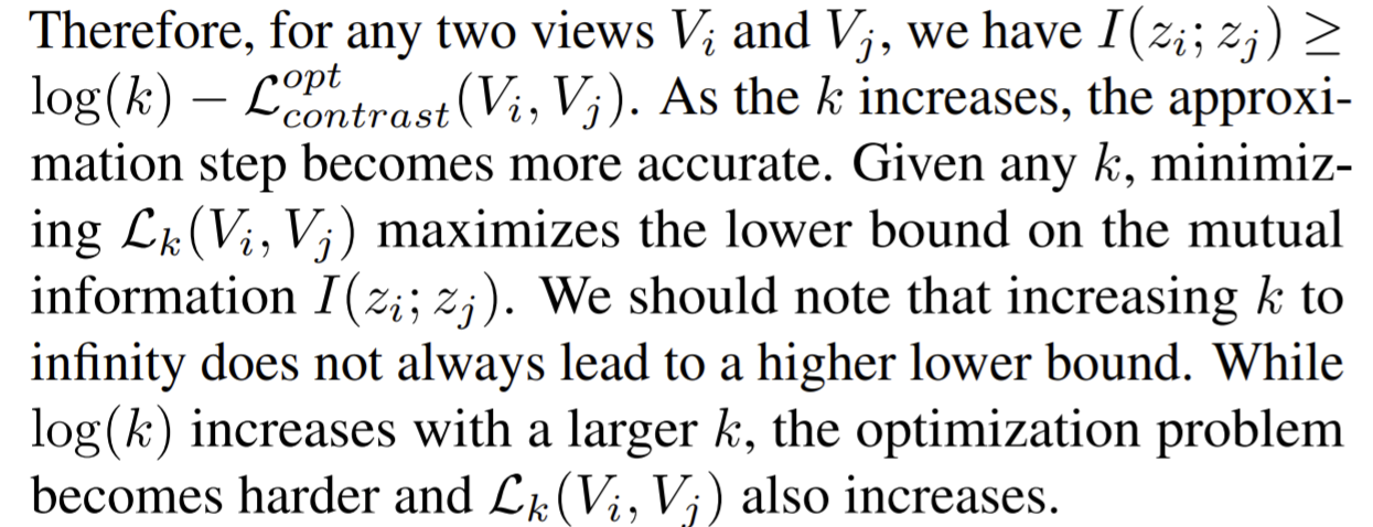
combining CMC with the MoCo mechanism or JigSaw branch in PIRL can consistently improve the performance, verifying that they are compatible.
Paper 8: Data-Efficient Image Recognition with Contrastive Predictive Coding (CPC v2: Improved CPC evaluated on limited labelled data)
Previous
CPC only requires in its definition that observations be ordered along e.g. temporal or spatial dimensions. It learns representations by training neural networks to predict the representations of future observations from those of past ones.
Loss

The loss is inspired by NCE, called as InfoNCE.
The negative samples \(\{z_l\}\) are taken from other locations in the image and other images in the mini-batch.
AMDIM is most similar to CPC in that it makes predictions across space, but differs in that it also predicts representations across layers in the model.
For improving data efficiency , one way is label-propogation.
- a classifier is trained on a subset of labeled data
- then used to label parts of the unlabeled dataset
Representation learning and label propagation have been shown to be complementary and can be combined to great effect (Zhai et al., 2019).
This work focus on representation learning.
What
- hypothesize that data-efficient recognition is enabled by representations which make the variability in natural signals more predictable
- removing low-level cues which might lead to degenerate solutions.
How
- Pretrain the encoder by CPC on local patches, and during test, apply the encoder on the entire image.
- Evaluation
- Linear classification: mean pooling followed by a single linear layer as the classifier. Use cross-entropy loss.
- Efficient classification: fix / fine tune the pretrained encoder, and then train the classifier (ResNet-33). Use a smaller learning rate and early-stopping for fine tuning incase the encoder deviates too much from the solution by the CPC objective.
- transfer learning: transfer the pretrained encoder to faster-RCNN to do classification. This is a multi-task.
- supervised training: directly train classifier by the input data, use cross-entropy loss.
Experiments
- Compare \(1\%\) supervised DNN based on CPC encoder with Semi-supervised methods and then supervised ResNets.
From CPC v1 to CPC v2
- Four axes for model capacity
- increasing depth and width: \(+5\%\). $+2% $ Top-1 accuracy with larger patches.
- improves training efficiency by importing layer normalization: can reclaim much of batch normalization’s training efficiency by using layer normalization (\(+2\%\) accuracy)
- making predictions in all four direction: Additional predictions tasks incrementally increased accuracy (adding bottom-up predictions: +2% accuracy; using all four spatial directions: +2.5% accuracy).
- perform patch-based augmentation: ‘color dropping’ (+3% accuracy); adding a fixed, generic augmentation scheme using the primitives from (shearing, rotation etc.), as well as random elastic deformations and color transforms +4.5% accuracy in total.
Efficient image classification
- fine-tune the entire stack hψ ◦ fθ for the supervised objective, for a small number of epochs (chosen by cross-validation)
- with only 1% of the labels, our classifier surpasses the supervised baseline given 5% of the labels
- the family of ResNet-50, -101, and -200 architectures are designed for supervised learning, and their capacity is calibrated for the amount of training signal present in ImageNet labels; larger architectures only run a greater risk of overfitting.
- fine-tuned representations yield only marginal gains over fixed ones
- we find that CPC provides gains in data efficiency that were previously unseen from representation learning methods, and rival the performance of the more elaborate label-propagation algorithms.
Transfer learning: image detection on PASCAL VOC 2007
- unsupervised pre-training surpasses supervised pretraining for transfer learning
Conclusion
- images are far from the only domain where unsupervised representation learning is important.
Paper 9: Momentum Contrast for Unsupervised Visual Representation Learning (MoCo, see also MoCo v2)
Have read MoCo before, here only list MoCo v2.
Previous
- Momentum Contrast (MoCo) shows that unsupervised pre-training can surpass its ImageNet-supervised counterpart in multiple detection and segmentation tasks.
- the negative keys are maintained in a queue, and only the queries and positive keys are encoded in each training batch.
- MoCo decouples the batch size from the number of negatives.
- SimCLR further reduces the gap in linear classifier performance between unsupervised and supervised pre-training representations.
- In an end-to-end mechanism, the negative keys are from the same batch and updated endto-end by back-propagation. SimCLR is based on this mechanism and requires a large batch to provide a large set of negatives.
What
- verify the effectiveness of two of SimCLR’s design improvements by implementing them in the MoCo framework
- using an MLP projection head and more data augmentation—we establish stronger baselines that outperform SimCLR and do not require large training batches.
How
- Evaluation
- ImageNet linear classification: features are frozen and a supervised linear classifier is trained
- Transferring to VOC object detection: a Faster R-CNN detector (C4-backbone) is fine-tuned end-to-end on the VOC 07+12 trainval set and evaluated on the VOC 07 test set using the COCO suite of metrics
- Amending
- replace the fc head in MoCo with a 2-layer MLP head (hidden layer 2048-d, with ReLU). This MLP only influences the unsupervised training stage; the linear classification or transferring stage does not use this MLP head.
- including the blur augmentation because stronger color distortion in A simple framework for contrastive learning of visual representations has diminishing gains in our higher baselines.
Experiments
- pre-training with the MLP head improves from 60.6% to 62.9%. in contrast to the big leap on ImageNet, the detection gains are smaller
- linear classification accuracy is not monotonically related to transfer performance in detection
- large batches are not necessary for good accuracy, and state-of-the-art results can be made more accessible.
Paper 10: A Simple Framework for Contrastive Learning of Visual Representations (SimCLR). ICML 2020
https://github.com/google-research/simclr
Previous
- Many such approaches have relied on heuristics to design pretext tasks, which could limit the generality of the learned representations.
- Types of augmentations
- spatial/geometric transformation of data: cropping and resizing (with horizontal flipping), rotation and cutout
- appearance transformation, such as color distortion (including color dropping, brightness, contrast, saturation, hue), Gaussian blur, and Sobel filtering.
- it is not clear if the success of contrastive approaches is determined by the mutual information, or by the specific form of the contrastive loss
What
- composition of multiple data augmentations plays a critical role in defining effective predictive tasks
- introducing a learnable nonlinear transformation between the representation and the contrastive loss substantially improves the quality of the learned representations
- contrastive learning benefits from larger batch sizes and more training steps compared to supervised learning
- Representation learning with contrastive cross entropy loss benefits from normalized embeddings and an appropriately adjusted temperature parameter.
How
SimCLR learns representations by maximizing agreement between differently augmented views of the same data example via a contrastive loss in the latent space.
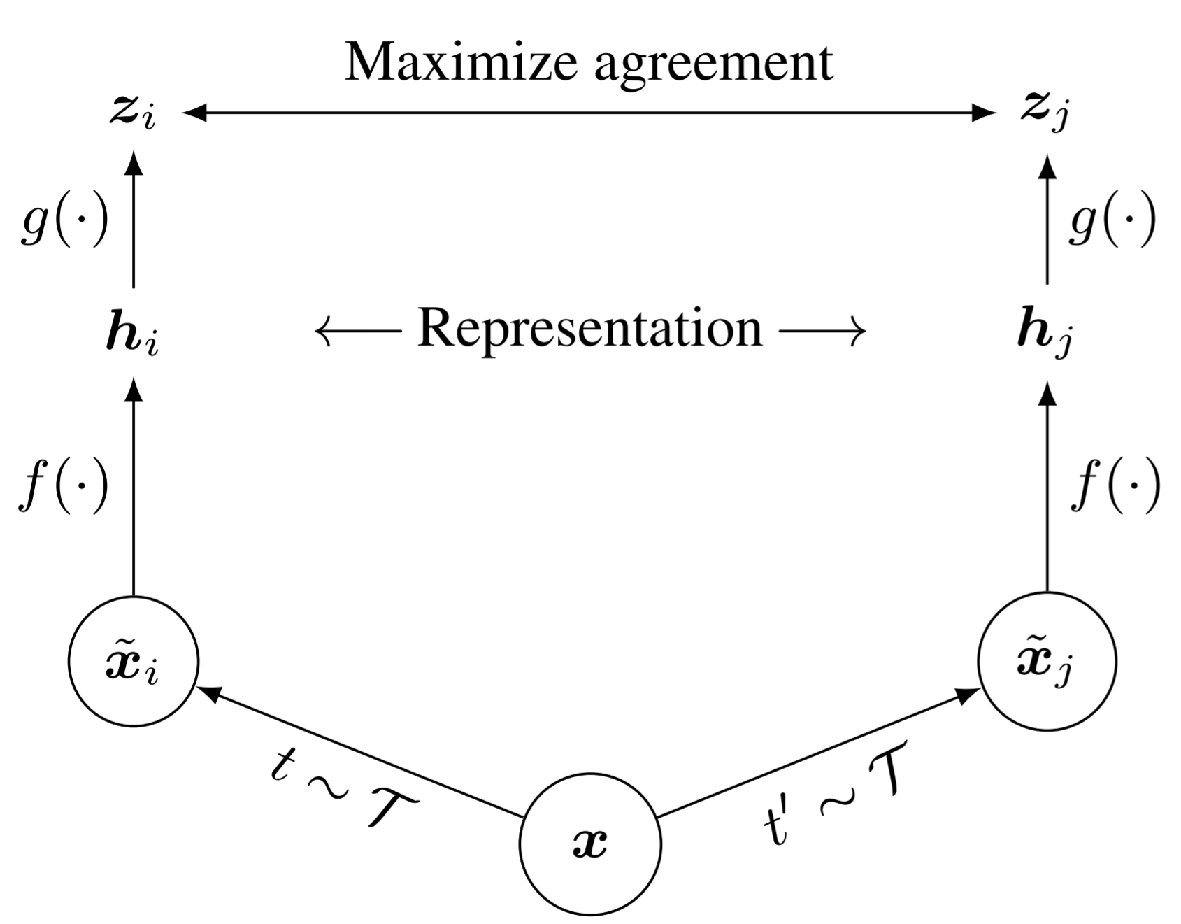
Where the \(x\) is the input data from one image, \(t\sim\mathcal{T}\) is the augmentation operator, and \(f(\cdot)\) is the encoder operator, \(g(\cdot)\) is the projection head. In downstream task, the \(h\) is used as the extracted features for classification.
- define the contrastive prediction task on pairs of augmented examples derived from the minibatch. Negative samples are not sampled explicitly.
- Use dot product as the similarity measurement. The final loss is termed as NT-Xent (the normalized temperature-scaled cross entropy loss).

- vary the training batch size N from 256 to 8192. A batch size of 8192 gives us 16382 negative examples per positive pair from both augmentation views. Since large batch size with SGD will induce to unstable, use LARS optimizer instead.
- as positive pairs are computed in the same device, use global BN by aggregating BN mean and variance over all devices during the training.
- shuffling data examples across devices, replacing BN with layer norm
Evaluation protocol
- Linear classifier, and compare with SOTA on Semi-supervised and transfer learning.
- default settings
- augmentation: random crop and resize (with random flip), color distortions, and Gaussian blur
- use ResNet-50 as the base encoder network
- a 2-layer MLP projection head to project the representation to a 128-dimensional latent space
- train at batch size 4096 for 100 epochs
- linear warmup for the first 10 epochs, and decay the learning rate with the cosine decay schedule without restarts
Experiments
Data augmentation
- Found no single transformation suffices to learn good representations
- One composition of augmentations stands out: random cropping and random color distortion
- Though color histograms alone suffice to distinguish images, most patches from an image share a similar color distribution.
- Stronger color augmentation substantially improves the linear evaluation of the learned unsupervised models. But for supervised methods, the stronger color augmentation even hurt the performance.==> unsupervised contrastive learning benefits from stronger (color) data augmentation than supervised learning
Architectures for encoder and head
- Unsupervised contrastive learning benefits (more) from bigger models
- the gap between supervised models and linear classifiers trained on unsupervised models shrinks as the model size increases,
- suggesting that unsupervised learning benefits more from bigger models than its supervised counterpart.
- training logger does not improve supervised methods.
- the gap between supervised models and linear classifiers trained on unsupervised models shrinks as the model size increases,
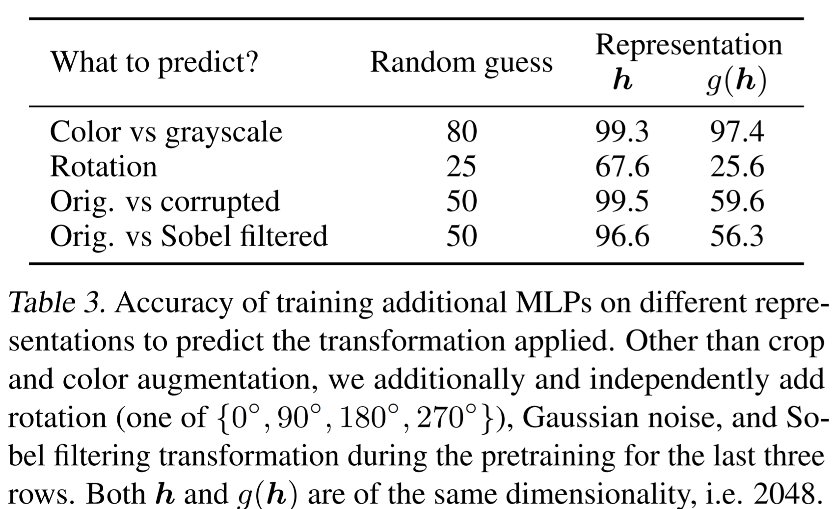
- A nonlinear projection head improves the representation quality of the layer before it
- a nonlinear projection is better than a linear projection (+3%), and much better than no projection (>10%)
- hidden layer before the projection head is a better representation than the layer after
- They explain this is due to loss of information induced by the contrastive loss
- \(g\) (projection head) can remove information that may be useful for the downstream task, such as the color or orientation of objects
Loss functions and batch size
- Normalized cross entropy loss with adjustable temperature works better than alternatives
- NT-Xent loss against such as logistic loss and margin loss.
- \(\ell_2\) normalization (i.e. cosine similarity) along with temperature effectively weights different examples, and an appropriate temperature can help the model learn from hard negatives
- unlike cross-entropy, other objective functions do not weigh the negatives by their relative hardness
- without normalization and proper temperature scaling, performance is significantly worse
- NT-Xent loss against such as logistic loss and margin loss.
- Contrastive learning benefits (more) from larger batch sizes and longer training
- when the number of training epochs is small (e.g. 100 epochs), larger batch sizes have a significant advantage over the smaller ones
- With more training steps/epochs, the gaps between different batch sizes decrease or disappear, provided the batches are randomly resampled
- Training longer also provides more negative examples, improving the results.
Learning rate and projection matrix
- square root learning rate scaling improves the performance for models trained with small batch sizes and in smaller number of epoch
- The linear projection matrix for computing \(z\) is approximately low rank, indicating by the plot of eigenvalues.
The way to train downstream classifier
attaching the linear classifier on top of the base encoder (with a stop_gradient on the input to linear classifier to prevent the label information from influencing the encoder) and train them simultaneously during the pretraining achieves similar performance
The best temperature parameter
- the optimal temperature in {0.1, 0.5, 1.0} is 0.5 and seems consistent regardless of the batch sizes.
Compared with SOTA
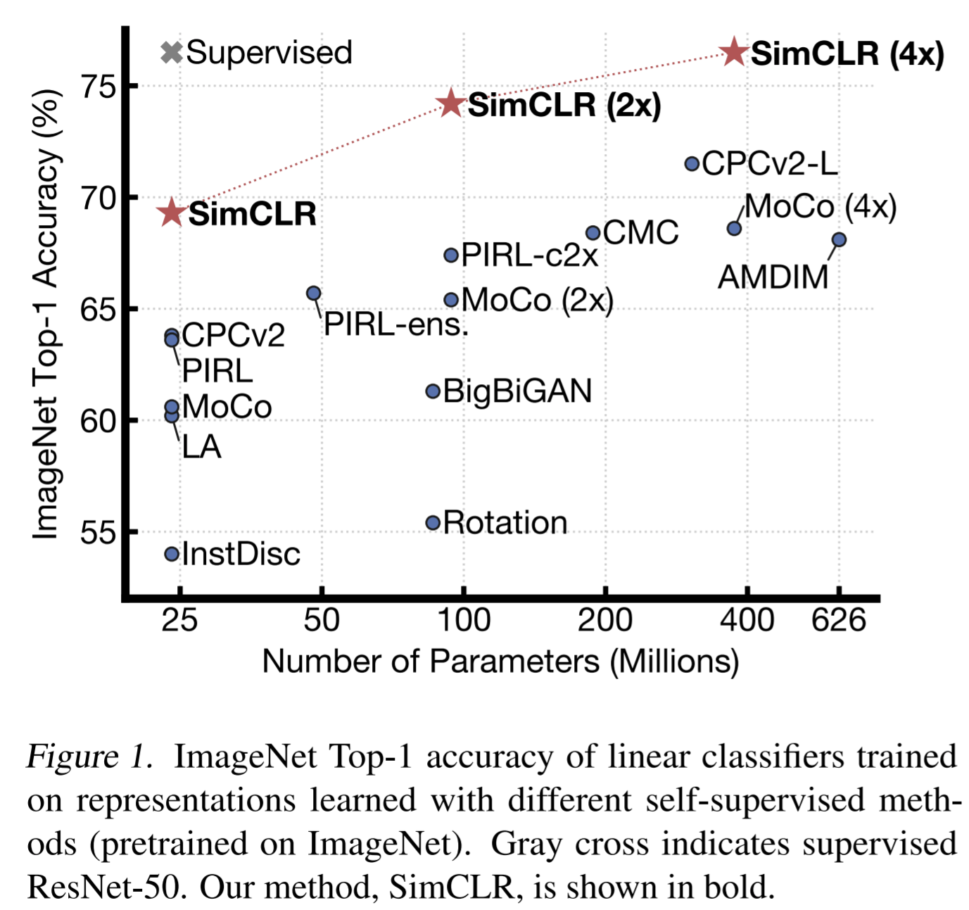
- fine-tuning our pretrained ResNet-50 (2×, 4×) on full ImageNet are also significantly better then training from scratch (up to 2%)
- our self-supervised model significantly outperforms the supervised baseline on 5 datasets, whereas the supervised baseline is superior on only 2
Paper 11: Big Self-Supervised Models are Strong Semi-Supervised Learners (SimCLRv2) ArXiv 2020
Previous
- semi-supervised learning involves unsupervised or self-supervised pretraining. It leverages unlabeled data in a task-agnostic way during pretraining, as the supervised labels are only used during fine-tuning.
- An alternative approach, directly leverages unlabeled data during supervised learning, as a form of regularization. uses unlabeled data in a task-specific way to encourage class label prediction consistency on unlabeled data among different models or under different data augmentations.
What
- Found the fewer the labels, the more this approach (task-agnostic use of unlabeled data) benefits from a bigger network
- The proposed semi-supervised learning algorithm in three steps:
- unsupervised pretraining of a big ResNet model using SimCLRv2,
- supervised fine-tuning on a few labeled examples,
- and distillation with unlabeled examples for refining and transferring the task-specific knowledge.
- make use of unlabeled data for a second time to encourage the student network to mimic the teacher network’s label predictions
How
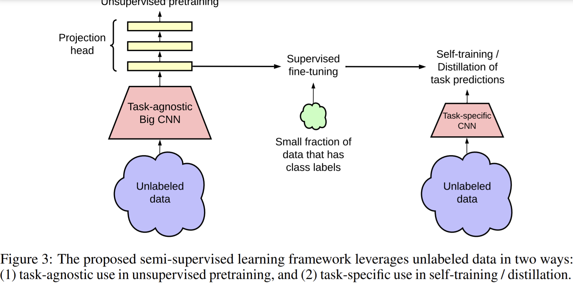
- train the student network by the labels predicted by the teacher network, also can add some real labels, while the student and teacher network are both trained by unlabeled data.
- SimCLR v2
- With bigger backbone (encoder): The largest model we train is a 152-layer ResNet [25] with 3× wider channels and selective kernels (SK). From ResNet-50 to ResNet-152 (3×+SK), we obtain a 29% relative improvement in top-1 accuracy when fine-tuned on 1% of labeled examples
- Increase the capacity of the projection head by making it deeper. Use a 3-layer projection head and fine tuning from the 1st layer of projection head. It results in as much as 14% relative improvement in top-1 accuracy when fine-tuned on 1% of labeled examples.
- Incorporate the memory mechanism from MoCo. It yields an improvement of ∼1% for linear evaluation as well as when fine-tuning on 1% of labeled examples when the SimCLR is trained in larger batch size.
- Fine-tuning
- Instead of throwing away the projection head directly, they fine-tune the model from a middle layer of the projection head, instead of the input layer of the projection head as in SimCLR.
- Self-training
- leverage the unlabeled data directly for the target task
- minimize the following distillation loss where no real labels are used:

- during distillation the teacher network is fixed.
- If do it in semi-supervised:

- The student model can be the same as the teacher or be smaller.
Experiments
- Benchmarks: ImageNet ILSVRC-2012. only a randomly sub-sampled 1% (12811) or 10% (128116) of images are associated with labels.
- with a batch size of 4096 and global batch normalization, for total of 800 epochs
- The memory buffer is set to 64K, use the same augmentations as in SimCLR v1, namely random crop, color distortion, and Gaussian blur.
- Two student networks, one is the same as the teacher, the other is smaller than the teacher to test the self-distillation and big-to-small distillation. Only random crop and horizontal flips of training images are applied during fine-tuning and distillation.
Bigger models are more label-efficient
- train ResNet by varying width and depth as well as whether or not to use selective kernels (SK). If use SK, they use the ResNet-D version.
- Use SK will cause larger model size.
- increasing width and depth, as well as using SK, all improve the performance. But the benefits of width will plateau.
- bigger models are more label-efficient for both supervised and semi-supervised learning, but gains appear to be larger for semi-supervised learning.
Bigger/deeper projection heads improve representation learning
- using a deeper projection head during pretraining is better when fine-tuning from the optimal layer of projection head, and this optimal layer is typically the first layer of projection head rather than the input (0th layer).
- when using bigger ResNets, the improvements from having a deeper projection head are smaller.
- it is possible that increasing the depth of the projection head has limited effect when the projection head is already relatively wide.
- Correlation is higher when fine-tuning from the optimal middle layer of the projection head than when fine-tuning from the projection head input, which indicates the accuracy of fine-tuned models is more related with the optimal middle layer of the projection head.
Distillation using unlabeled data improves semi-supervised learning
Two loss: distillation loss and an ordinary supervised cross-entropy loss on the labels.
Using the distillation loss alone works almost as well as balancing distillation and label losses when the labeled fraction is small (1%, 10%).
To get the best performance for smaller ResNets, the big model is self-distilled before distilling it to smaller models
when the student model has a smaller architecture than the teacher model, it improves the model efficiency by transferring task-specific knowledge to a student model; even when the student model has the same architecture as the teacher model (excluding the projection head after ResNet encoder), self-distillation can still meaningfully improve the semi-supervised learning performance.
task-agnostically learned general representations can be distilled into a more specialized and compact network using unlabeled examples.
The benefits are larger when (1) regularization techniques (such as augmentation, label smoothing) are used, or (2) the model is pretrained using unlabeled examples
a better fine-tuned model (measured by its top-1 accuracy), regardless their projection head settings, is a better teacher for transferring task specific knowledge to the student using unlabeled data.
Paper 12: Unsupervised Learning of Visual Features by Contrasting Cluster Assignments (SwAV) ArXiv 2020
https://github.com/facebookresearch/swav
Previous
- contrastive methods typically work online and rely on a large number of explicit pairwise feature comparisons, which is computationally expensive.
- In contrastive methods, the loss function and augmentations both contribute to the performance.
- most implementations approximate the loss by reducing the number of comparisons to random subsets of images during training
- An alternative to approximate the loss is to approximate the task—that is to relax the instance discrimination problem. E.g., clustering-based methods discriminate between groups of images with similar features instead of individual images. But it does not scale well with the dataset as it requires a pass over the entire dataset to form image “codes” (i.e., cluster assignments) that are used as targets during training.
- Amendment: They avoid comparing every pair of images by mapping the image features to a set of trainable prototype vectors.
- Typical clustering-based methods are offline in the sense that they alternate between a cluster assignment step where image features of the entire dataset are clustered, and a training step where the cluster assignments, i.e., “codes” are predicted for different image views.
What
- propose an online algorithm, SwAV, that takes advantage of contrastive methods without requiring to compute pairwise comparisons. Their method can be interpreted as a way of contrasting between multiple image views by comparing their cluster assignments instead of their features.
- simultaneously clusters the data while enforcing consistency between cluster assignments produced for different augmentations (or “views”) of the same image
- predict the code of a view from the representation of another view, and called it as swapped assignments between multiple views of the same image (SwAV)
- memory efficient since it does not require a large memory bank or a special momentum network.
- Propose multi-crop as a new augmentation, uses a mix of views with different resolutions in place of two full-resolution views. It consists in simply sampling multiple random crops with two different sizes: a standard size and a smaller one.
- mapping small parts of a scene to more global views significantly boosts the performance.
- Use ResNet as the backbone and ImageNet as the benchmark.
How
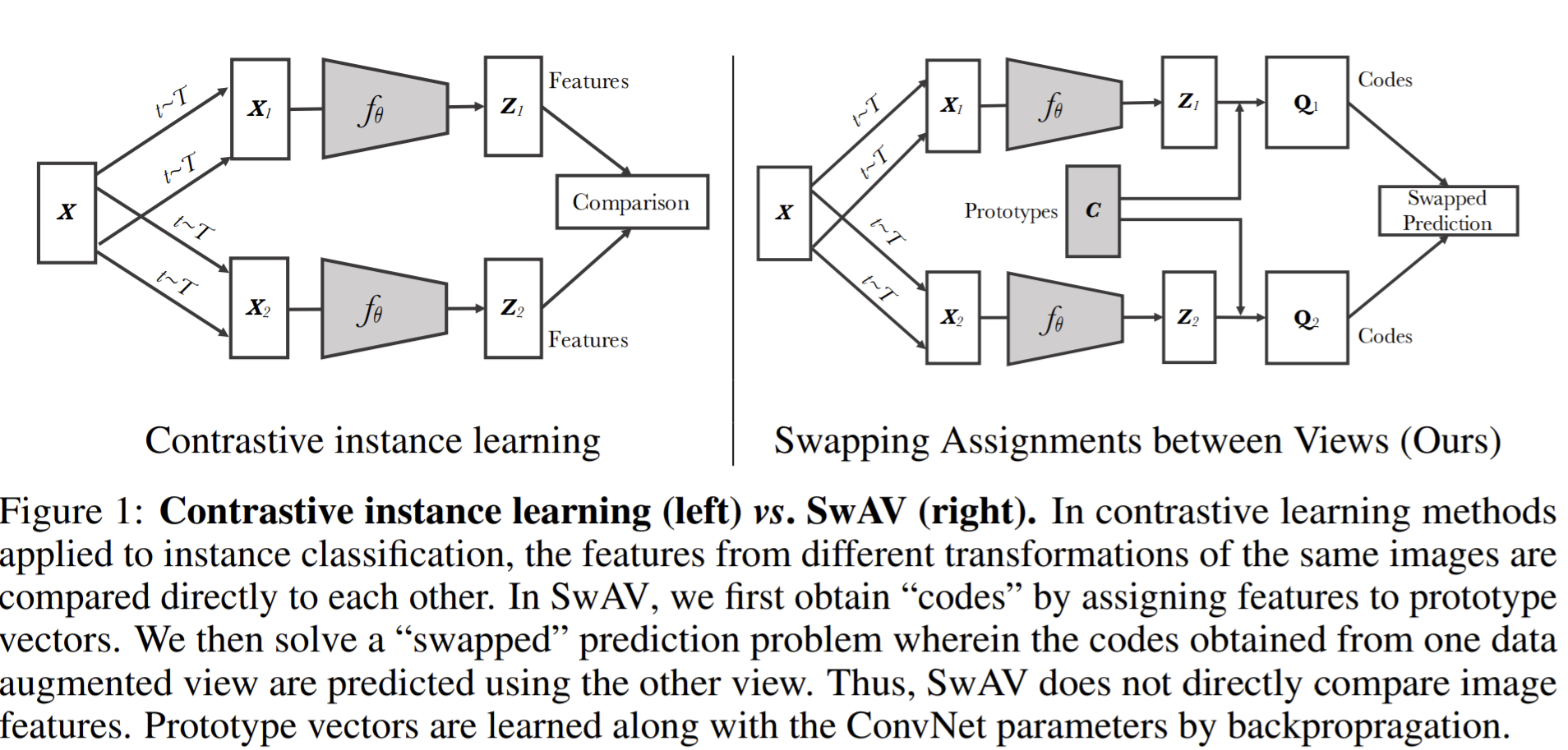
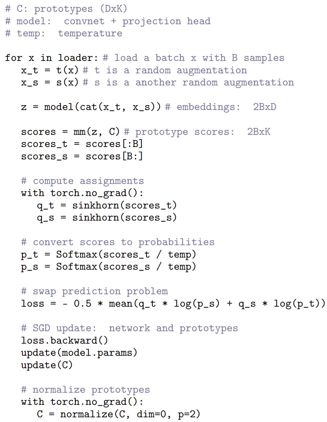
Prototype vectors \(C\) are learned along with the ConvNet parameters by backpropragation, and they are mapped with the predicted \(z\) to search the codes \(Q\).
- For two image features \(z_t,z_s\), predict the codes \(q_t,q_s\), the the loss is \(L(z_t,z_s)=\ell(z_t,q_s)+\ell(z_s,q_t)\). \(\ell(z,q)\) measures the fit between features \(z\) and a code \(q\). \(\ell(z_t,q_s)=-\sum_k q_s^{(k)}\log p_t^{(k)}\), where \(p_t^{(k)}=\frac{\exp{(\frac{1}{\tau}}z_t^Tc_k)}{\sum_{k'}\exp{(\frac{1}{\tau}z_t^Tc_{k'}})}\).

Online codes computing: to get the soft predicted codes \(Q^*\)
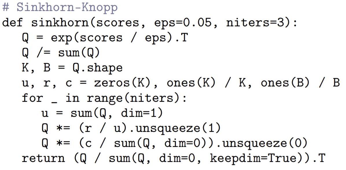
- optimize \(Q\) to maximized the similarity between the features and the prototypes, i.e.,


- the entropy \(H(Q)\) controls the diversity of the codes, and a strong entropy regularization (i.e. using a high ε) generally leads to a trivial solution where all samples collapse into an unique representation and are all assigned uniformely to all prototypes. They keep \(\varepsilon\) small.
- Enforce that on average each prototype is selected at least \(\frac{B}{K}\) times in the batch.
- In online version, the continuous codes work better than discrete codes (rounding the continuous codes)
- An explanation is that the rounding needed to obtain discrete codes is a more aggressive optimization step than gradient updates. While it makes the model converge rapidly, it leads to a worse solution.
- The soft codes \(Q^*\) is
 , where \(u,v\) are renormalization vectors in \(\mathbb{R}^K, \mathbb{R}^B\) respectively (prototypes and feature space).
 - In practice, we observe that using only 3 iterations is fast and sufficient to obtain good performance for solving \(Q^*\).
- When working with small batches, we use features from the previous batches to augment the size of \(Z\) to equally partition the batch into the \(K\) prototypes. Then, we only use the codes of the batch features in our training loss
- optimize \(Q\) to maximized the similarity between the features and the prototypes, i.e.,
In practice, the size of keep batches
- we store around 3K features, i.e., in the same range as the number of code vectors.
- we only keep features from the last 15 batches with a batch size of 256, while contrastive methods typically need to store the last 65K instances obtained from the last 250 batches
Multi-crop
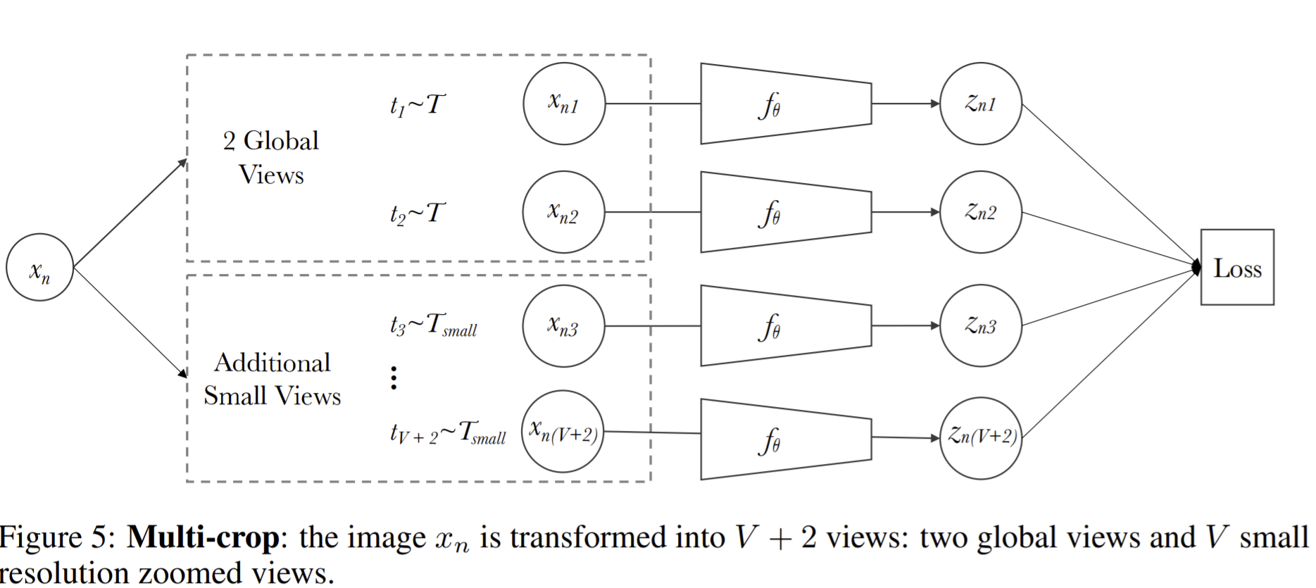
- use two standard resolution crops and sample \(V\) additional low resolution crops that cover only small parts of the image. The low resolution is for computation efficiency.

- We compute codes \(q\) using only the full resolution crops. using only partial information (small crops cover only small area of images) degrades the assignment quality
- Why \(i=\{1,2\}\) here? Because for each image, apply \(s,t\) transformations? And swap just swap the predicted codes for the same source images (\(x_s,x_t\)).
Experiments
main results
SwAV is not specifically designed for semi-supervised learning
Outperform other Self-supervised methods if using frozen features.
The performance of our model increases with the width of the model, and follows a similar trend to the one obtained with supervised learning
one epoch of MoCov2 or SimCLR is faster in wall clock time than one of SwAV, but these methods need more epochs for good downstream performance.
Clustering-based SSL
- In DeepCluster-v2, instead of learning a classification layer predicting the cluster assignments, we perform explicit comparison between features and centroids.
- SwAV and DeepCluster-v2 outperform SimCLR by 2% without multi-crop and by 3.5% with multi-crop.
- DeepCluster-v2 is not online which makes it impractical for extremely large datasets. DeepCluster-v2 can be interpreted as a special case of our proposed swapping mechanism: swapping is done across epochs rather than within a batch.
Multi-crop to different methods: multi-crop seems to benefit more clustering-based methods than contrastive methods. We note that multi-crop does not improve the supervised model
Longer training: While SwAV benefits from longer training, it already achieves strong performance after 100 epochs.
Unsupervised pretraining on a large uncurated dataset
- evaluate SwAV on random, uncurated images that have different properties from ImageNet which allows us to test if our online clustering scheme and multi-crop augmentation work out of the box: pretrain SwAV on an uncurated dataset of 1 billion random public non-EU images from Instagram. Then the trained model is used to evaluate ImageNet task.
- SwAV maintains a similar gain of 6% over SimCLR as when pretrained on ImageNet==> our improvements do not depend on the data distribution
- Capacity
- SwAV outperforms training from scratch by a significant margin showing that it can take advantage of the increased model capacity.
Other results
- start using a queue composed of the feature representations from previous batches after 15 epochs of training.
- the prototypes in SwAV are not strongly encouraged to be categorical and random fixed prototypes work almost as well==> they help contrasting different image views without relying on pairwise comparison with many negatives samples.
Paper 13: What Should Not Be Contrastive in Contrastive Learning ArXiv 2020
Previous
- The methods of SSL contrastive methods assume a particular set of representational invariances.
- The property of contrastive sampling like in MoCo negatively affects the learnt representations:
- Generalizability and transferability are harmed if they are applied to the tasks where the discarded information is essential, e.g., color plays an important role in fine-grained classification of birds;
- Adding an extra augmentation is complicated as the new operator may be helpful to certain classes while harmful to others, e.g., a rotated flower could be very similar to the original one, whereas it does not hold for a rotated car;
- The hyper-parameters which control the strength of augmentations need to be carefully tuned for each augmentation to strike a delicate balance between leaving a short-cut open and completely invalidate one source of information.
What
- introduce a contrastive learning framework which does not require prior knowledge of specific, task-dependent invariances. The model learns to capture varying and invariant factors for visual representations by constructing separate embedding spaces, each of which is invariant to all but one augmentation.
- We use a multi-head network with a shared backbone which captures information across each augmentation and alone outperforms all baselines on downstream tasks.
- does not require hand-selection of data augmentation strategies, and achieves better performance against state-of-the-art MoCo baseline
- Propose LOOC (leave-one-out contrastive learning).
How
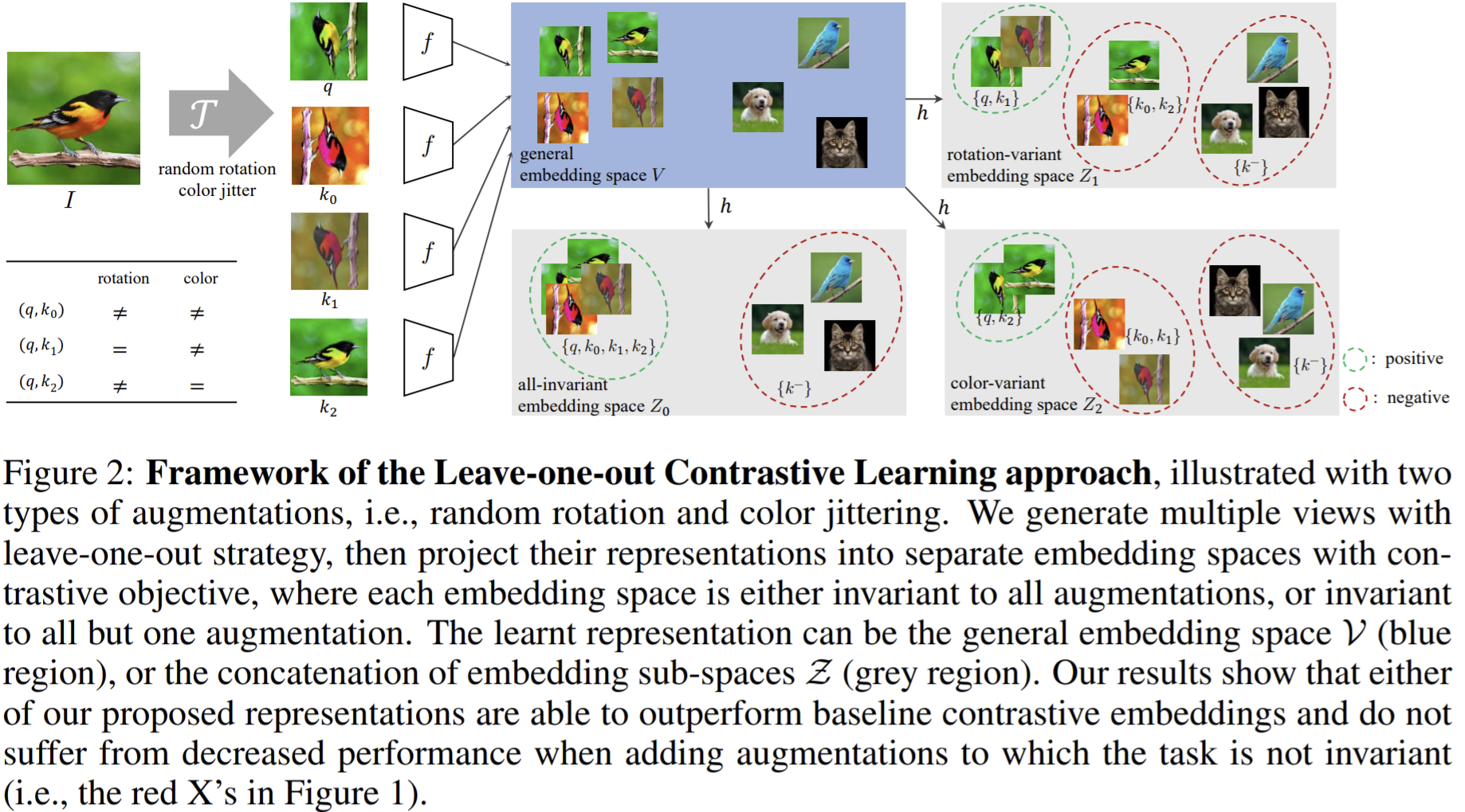

- \(\mathcal{Z}_i\) is dependent on the \(i^{th}\) type of augmentation but invariant to other types of augmentations.
- In \(\mathcal{Z}_0\), all features \(v\) should be mapped to a single point
- In \(\mathcal{Z}_i\), only \(v^q,v^{k_i}\) should be mapped to a single point while \(v^{k_j} \forall j\neq i\) should be mapped to \(n-1\) separate points.
- Use MoCo as the framework, and ResNet50 as backbone. Use augmentations: color jittering (including random gray scale), random rotation (90,180,or 270) and texture randomization.
- Use random-resized croppping, horizontal flipping and Gaussian blur as augmentations without designated embedding space.
- In LooC++, use the concatenation of the output of Conv5 and the last layer of \(h\) from each head to build a new input for the projection head.
- After training, we adopt linear classification protocol by training a supervised linear classifier on frozen features of feature space \(\mathcal{V}\) for LooC, or concatenated feature spaces \(\mathcal{Z}\) for LooC++.
Experiments
- Test on In-100 validation set, the iNaturalist (iNat-1k) dataset, VGG flowers, ObjectNet and ImageNet-C.
- Use two-layer MLP head with a 2048-d hidden later and ReLU for each individual embedding space.
- Inductive augmentation: Adding rotation augmentation into baseline MoCo significantly reduces its capacity to classify rotation angles while downgrades its performance on IN-100.
- In contrast, our method better leverages the information gain of the new augmentation.
- We can include all augmentations with our LooC multi-self-supervised method and obtain improved performance across all condition without any downstream labels or a prior knowledged invariance
- Fine-grained recognition results
- MoCo has marginally superior performance on IN-100
- But the original MoCo trails our LooC counterpart on all other datasets by a noticeable margin
- our method can better preserve color information.
- Rotation augmentation also boosts the performance on iNat-1k and Flowers-102, while yields smaller improvements on CUB-200, which supports the intuition that some categories benefit from rotation-invariant representations while some do not
- The performance is further boosted by using LooC with both augmentations ==> the effectiveness in simultaneously learning the information w.r.t. multiple augmentations
- the benefits of explicit feature fusion without hand-crafting what should or should not be contrastive in the training objective
- Robustness learning results
- The fully supervised network is most sensitive to perturbations
- The rotation augmentation is beneficial for ON-13, but significantly downgrades the robustness to data corruptions in IN-C-100.
- texture randomization increases the robustness on IN-C-100 across all corruption types
- Combining rotation and texture augmentation yields improvements on both datasets
- Multiple heads
- Using multiple heads boosts the performance of baseline MoCo
- our method achieves better or comparable results compared with its baseline counterparts.
- Ablation of augmentation
- Textures are (overly) strong cues for ImageNet classification (Geirhos et al., 2018), thus the linear classifier is prone to use texture-dependent features, loosing the gains of texture invariance
- By checking the histograms of correct predictions (activations x weights of classifier). The classifier on IN-100 heavily relies on texture-dependent information, whereas it is much more balanced on iNat-1k.
- when human or animal faces dominant an image ((a), bottom-left), LooC++ sharply prefers rotation-dependent features, which also holds for face recognition of humans.
Paper 14: Self-Supervised Learning of Pretext-Invariant Representations. CVPR 2020
Previous
- Pre-defined semantic annotations scale poorly to the long tail of visual concepts, while SSL tries to address this problem.
- Representations ought to be invariant under image transformations to be useful for image recognition, because the transformations do not alter visual semantics.
What
- focuses on image-based pretext tasks
- Hint: semantic representations ought to be invariant under such transformations.==> we develop Pretext-Invariant Representation Learning (PIRL, pronounced as “pearl”) that learns invariant representations based on pretext tasks
- PIRL outperforms supervised pre-training in learning image representations for object detection.
- adapt the “Jigsaw” pretext task to work with PIRL
- PIRL even outperforms supervised pre-training in learning image representations suitable for object detection
- PIRL can be viewed as extending the set of data augmentations to include prior pretext tasks and provides a new way to combine pretext tasks with contrastive learning.
How
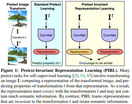
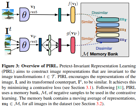
adopt the existing Jigsaw pretext task in a way that encourages the image representations to be invariant to the image patch perturbation
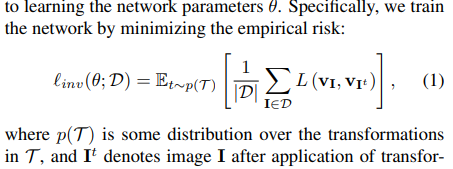
Use NCE to control the similarity between the features of \(I\) and the augmented patches of \(I_t\).

apply different “heads” to the features before computing the score

Use memory bank
- The representation \(m_I\) in memory bank is an exponential moving average of feature representations \(f(v_I)\) that were computed in prior epochs.
Final loss

- The first term is the equation above, and the second term encourages the representation \(f(v_I)\) to be similar to its memory representation so to control the parameters updating; and encourages the representations \(f(v_I),f(v_{I'})\) to be dissimilar.
Backbone: ResNet50
Representations
- \(f(v_I)\) from \(I\) is by extracting res5 features, average pooling and a linear projection to obtain a 128-dimensional representation.
Experiments
- Compare between PIRL (\(\lambda =0.5\)): NPID (\(\lambda =0\)) and NPID++ (with more negative samples, (\(\lambda =0\)) by setting \(\lambda\) in final loss.
Tasks
- Object detection
- benchmark: Pascal VOC
- encoder: faster RCNN C4 object detection model implement in detectron 2 with a ResNet-50.
- The success of PIRL underscore the importance of learning invariant (rather than covariant) image representations.
- a self-supervised learner can outperform supervised pre-training for object detection.
- PIRL learns image representations that are amenable to sample-efficient supervised learning.
- Image classification with linear models
- PIRL outperforms all prior self-supervised learners on ImageNet in terms of the trade-off between model accuracy and size. Indeed, PIRL even outperforms most self-supervised learners that use much larger models
- PIRL sets a new state-of-the-art for self-supervised representations in this learning setting on the VOC07, Places205, and iNaturalist datasets, while NPID++ performs well but is consistently outperformed by PIRL.
- Semi-supervised: finetuning the models on just 1% (∼13,000) labeled images leads to a top-5 accuracy of 57%.
- If pretrained on another unlabeled dataset and then test on ImageNet, PIRL even outperforms Jigsaw and DeeperCluster models that were trained on 100× more data from the same distribution.
- Other discussion
- Does PIRL learn invariant representations? for PIRL, an image representation and the representation of a transformed version of that image are generally similar, measured by the histogram of distance of normalized features \(f(v_I), g(v_{I_t})\).
- Which layer produces the best representations?
- the quality of Jigsaw representations improves from the conv1 to the res4 layer but that their quality sharply decreases in the res5 layer==> surmise this happens because the res5 representations in the last layer of the network covary with the image transformation t and are not encouraged to contain semantic information.
- , the best image representations are extracted from the res5 layer of PIRL-trained networks
- learning invariance to Jigsaw is important for better representations
- Loss functions
- At λ= 1, the network does not compare untransformed images at training time and updates to the memory bank \(m_I\) are not dampened
- The performance of PIRL is sensitive to the setting of λ, and the best performance is obtained by setting λ= 0.5
- Effect of the number of image transforms
- PIRL outperforms Jigsaw for all cardinalities of T . PIRL particularly benefits from being able to use very large numbers of image transformations (i.e., large |T |) during training
- Effect of the number of negative samples: increasing the number of negatives tends to have a positive influence on the quality of the image representations constructed by PIRL.
Paper 15 Adversarially Learned Inference (ALI) ICLR 2017
https://github.com/IshmaelBelghazi/ALI
Previous
- three classes of algorithms for learning deep directed generative models, in practice they learn very different kinds of generative models on typical datasets.
- VAE: suffer from the issue of the maximum likelihood training paradigm when combined with a conditional independence assumption on the output given the latent variables==> image samples from VAE-trained models tend to be blurry
- GANs: lack an efficient inference mechanism and thus cannot well reason about data at an abstract level.
- autoregressive models: can produce good samples but in slow sampling speed and foregoing the learning of an abstract representation of the data
- Feedforward inference in GANs
- InfoGAN: minimizes the mutual information between a subset \(c\) of the latent code and \(x\) through the use of an auxiliary distribution \(Q(c | x)\). But there are no inference of \(c\) and requires \(Q(c | x)\) to be tractable.
- But the inverse mapping is not well learned. If decompose into two phases to train the encoder and decoder, the GAN’s decoder is frozen and an encoder is trained following the ALI procedure (i.e., a discriminator taking both x and z as input is introduced). We call this post-hoc learned inference.
What
- Introduce ALI (adversarially learned inference) jointly learns a generation network and an inference network using an adversarial process
- Train the encoder (\(x\rightarrow z\)) and decoder (\(z\rightarrow x\)), these two are both the generator.
- The discriminator is trained to distinguish between joint pairs \((x, \hat{z} = G_x(x))\) and \((\tilde{x} = G_x(z), z)\), as opposed to marginal samples \(x ∼ q(x)\) and \(\tilde{x} ∼ p(x)\) in original GAN.
How
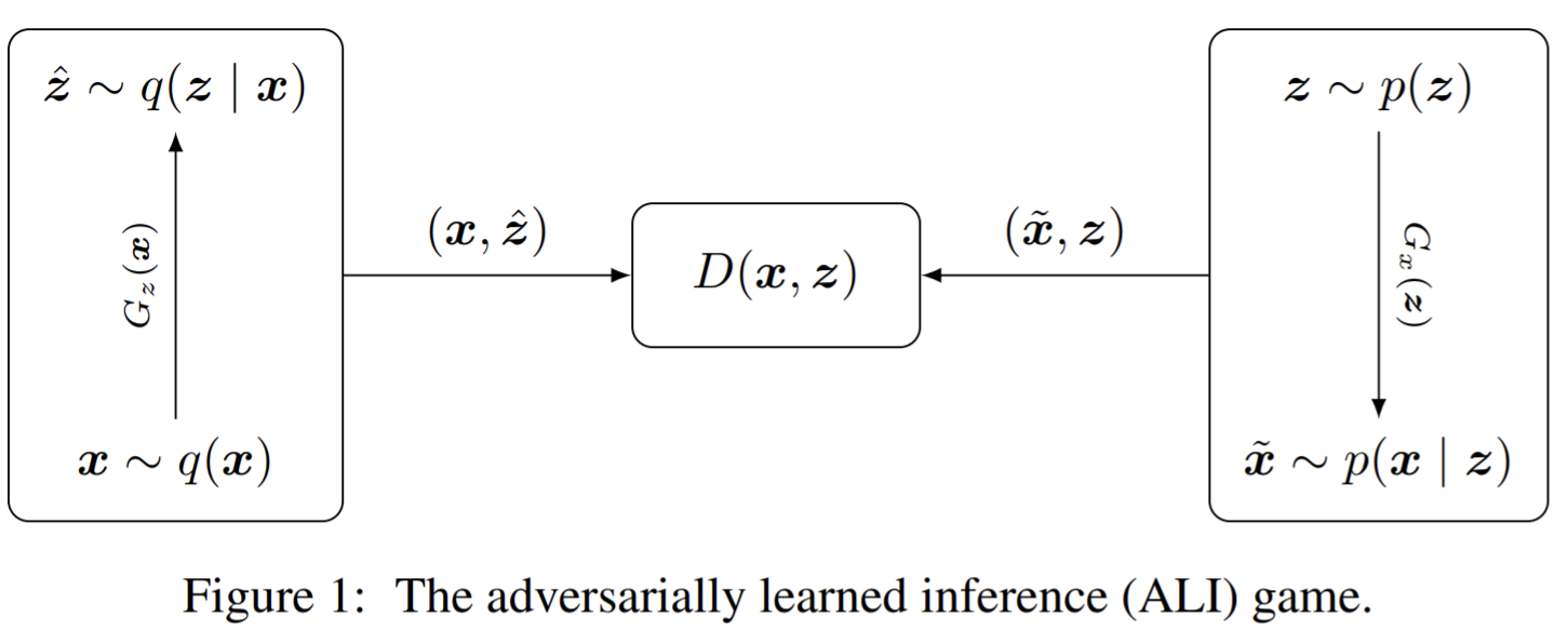
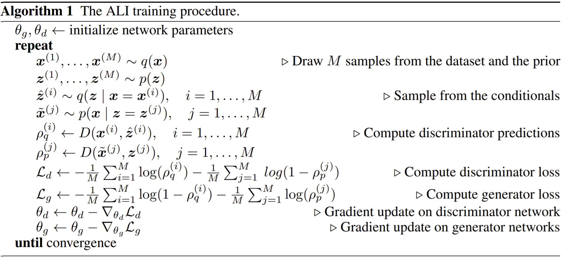
- For instance, if \(q(z | x) = \mathcal{N} (µ(x), σ^2 (x)I)\), one can draw samples by computing: \(z = µ(x) + σ(x) \bigodot \epsilon , \epsilon ∼ \mathcal{N} (0, I)\).
- As a workaround, the generator is trained to maximize:
 which has the same fixed points but whose gradient is stronger when the discriminator’s output saturates.
 - ALI is not directly applicable to either applications with discrete data or to models with discrete latent variables.
- The discriminator
Experiments
- Benchmarks: SVHN (Street View House Numbers), CIFAR-10, CelebA and a downsampled version of the ImageNet dataset.
- Found reconstructions are not always faithful reproductions of the inputs. They retain the same crispness and quality characteristic to adversarially-trained models, but oftentimes make mistakes in capturing exact object placement, color, style and (in extreme cases) object identity
- ALI is not concentrating its probability mass exclusively around training examples, but rather has learned latent features that generalize well
- ALI did not require feature matching to obtain comparable results. Latent representation learned by ALI is better untangled with respect to the classification task and that it generalizes better.
- The ALI encoder models a marginal distribution \(q(z)\) that matches \(p(z)\) fairly well (row 2, column a), while the GAN generator has more trouble reaching all the modes than the ALI generator.
- Learning an inverse mapping from GAN samples does not work very well. reconstructions suffer from the generator dropping modes.
- Learning inference post-hoc doesn’t work as well as training the encoder and the decoder jointly.
- this experiment provides evidence that adversarial training benefits from learning an inference mechanism jointly with the decoder.
Paper 16: Adversarial Feature Learning (BiGAN, concurrent and similar to ALI) ICLR 2017
Previous
- Way to learn inverse mapping
- directly model \(p(z|G(z))\), predicting generator input \(z\) given generated data \(G(z)\).
- The BiGAN that they proposed.
- GAN model the data distribution as a transformation of a fixed latent distribution \(p_Z(z)\) for \(z \in Ω_Z\), and the transformation is named as the generator.
- The ideal discriminator of vanilla GAN is equivalent to the Jensen-Shannon divergence between the two distributions \(p_G, p_x\).
What
- learn the inverse mapping – projecting data back into the latent space.
- propose Bidirectional Generative Adversarial Networks (BiGANs) as a means of learning this inverse mapping
How
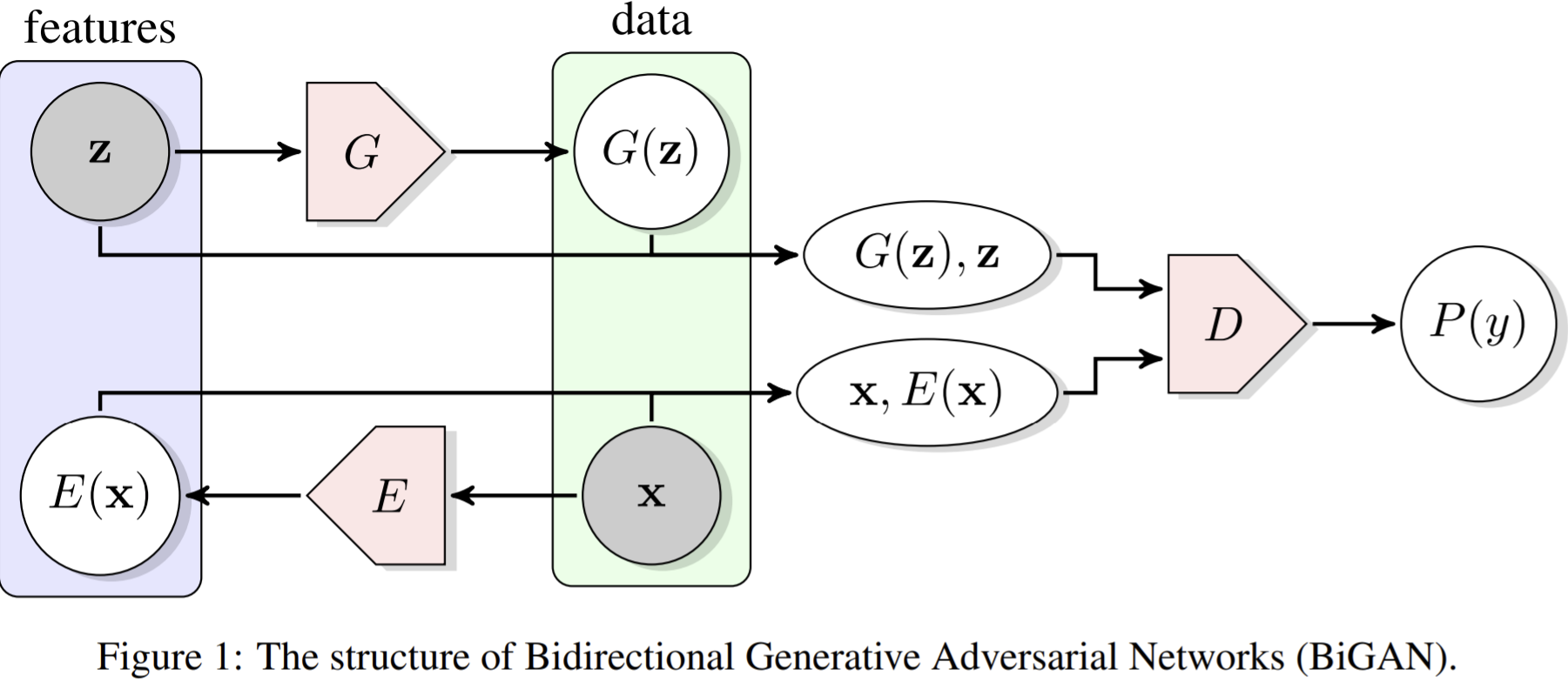
Include the generator G and the encoder E.
- a trained BiGAN encoder may serve as a useful feature representation for related semantic tasks, similar as what's obtained in the SSL.

The optimal discriminator, generator and decoder.

With the optimal discriminator, then


The optimal generator & encoder are inverses:

But these two are rarely exact inverses,while they two are approximate inverses.
BiGAN is closely related to AEs with an \(\ell_0\) loss.

- \(1_{[G(E(x))=x]}\) in the first term is equivalent to an autoencoder with \(\ell_0\) loss, while the indicator \(1_{[G(E(z))=z]}\) in the second term shows that the BiGAN encoder must invert the generator.
- Also the \(\ell_0\) loss does not make any assumptions about the structure or distribution of the data itself.
BiGAN optimizes a Jensen-Shannon divergence between a joint distribution over both data \(X\) and latent features \(Z\). This joint divergence allows us to further characterize properties of \(G\) and \(E\), as shown below.
Learning process:
- first the D is updated and then E and G are updated together.
- BiGAN training that an “inverse” objective provides stronger gradient signal to G and E (the real and generated labels Y are swapped).
- update all modules D, G, and E simultaneously at each iteration, rather than alternating between D updates and G, E updates
If \(G\) successfully generates the true data distribution \(p_X(x)\), D may ignore the input data entirely and predict \(P(Y = 1) = P(Y = 1|x) = \frac{1}{2}\) unconditionally, not learning any meaningful intermediate representations.
Experiments
- Evaluate on n both permutation-invariant MNIST and on the high-resolution natural images of ImageNet.
- in the all column, the entire network is “fine-tuned”
- Encoder E follows AlexNet, and D also.
- Found filters learned by the encoder E have clear Gabor-like structure, similar to those originally reported for the fully supervised AlexNet model
Paper 17: Large Scale Adversarial Representation Learning (Big BiGAN) ArXiv 2019
https://tfhub.dev/s?publisher=deepmind&q=bigbigan
https://colab.research.google.com/github/tensorflow/hub/blob/master/examples/colab/bigbigan_with_tf_hub.ipynb
Previous
- BiGAN behaves like an autoencoder minimizing \(\ell_0\) reconstruction costs; however, the shape of the reconstruction error surface is dictated by a parametric discriminator, as opposed to simple pixel-level measures like the \(\ell_2\) error.==> it will induce an error surface which emphasizes “semantic” errors in reconstructions, rather than low-level details.
- BiGAN used a DCGAN style generator, incapable of producing high-quality images on this dataset, so the semantics the encoder could model were in turn quite limited.
What
- Based on BiGAN, adding an encoder and modifying the discriminator
- demonstrating that these generation-based models achieve the state of the art in unsupervised representation learning on ImageNet, as well as in unconditional image generation
- The contributions
- We show that BigBiGAN (BiGAN with BigGAN generator) matches the state of the art in unsupervised representation learning on ImageNet.
- We propose a more stable version of the joint discriminator for BigBiGAN.
- We perform a thorough empirical analysis and ablation study of model design choices.
- We show that the representation learning objective also improves unconditional image generation, and demonstrate state-of-the-art results in unconditional ImageNet generation.
- We open source pretrained BigBiGAN models on TensorFlow Hub.
How
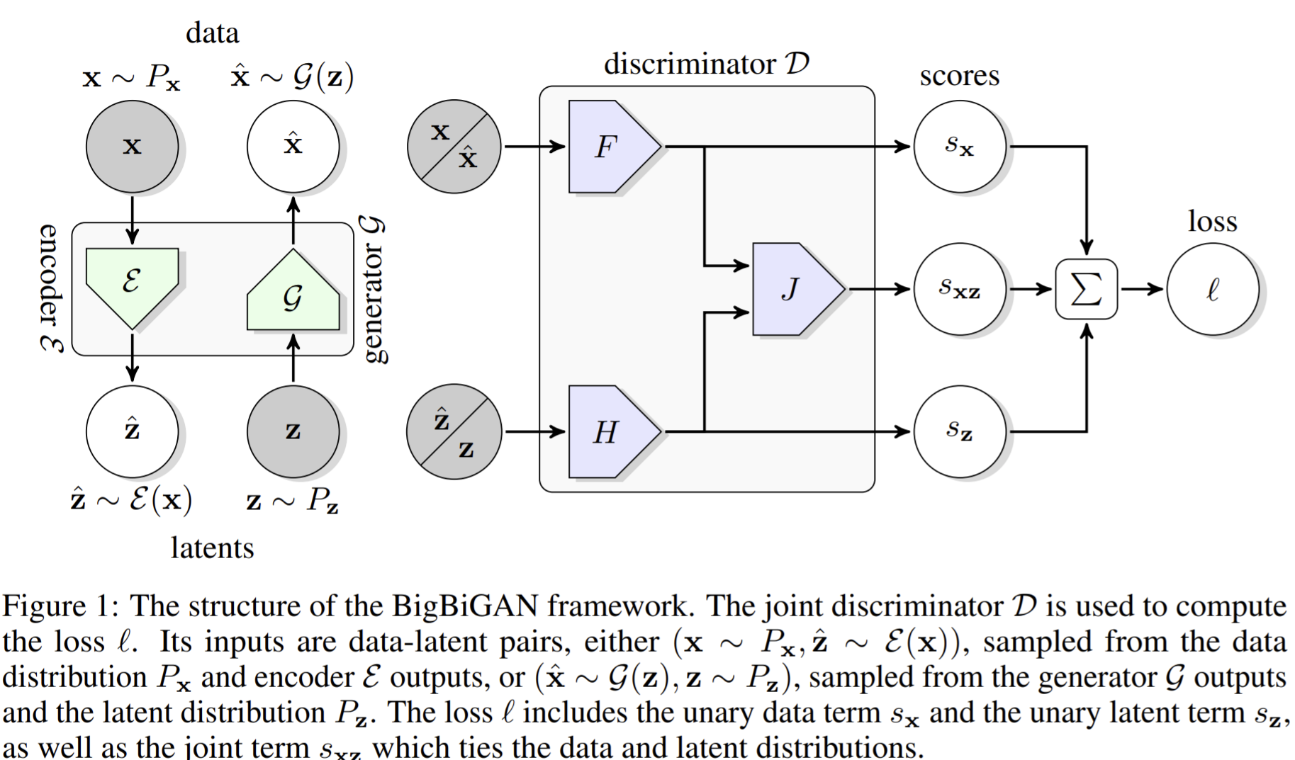
- Modifications of BiGAN:
- a joint discriminator D, which takes as input data-latent pairs \((x, z)\) (rather than just data \(x\) as in a standard GAN)
 where \(h(t)=\max (0,1-t)\) is a hinge used to regularize the discriminator.
- F is a convNet, H is an MLP, and J is the function of the outputs of F and H.
- The discriminator loss \(\mathcal{L}_D\) intuitively trains the discriminator to distinguish between the two joint data-latent distributions from the encoder and the generator, pushing it to predict positive values for encoder input pairs \((x, E(x))\) and negative values for generator input pairs \((G(z), z)\).
- train a BigBiGAN on unlabeled ImageNet, freeze its learned representation, and then train a linear classifier on its outputs, fully supervised using all of the training set labels
Experiments
- components of D – H and J – are 8-layer MLPs with ResNet-style skip connections (four residual blocks with two layers each) and size 2048 hidden layers
- Ablation
- latent distribution \(P_z\) and stochastic \(\mathcal{E}\): the non-deterministic \(\mathcal{E}\) model achieves significantly better classification performance (at no cost to generation)
- Unary loss terms \(s_x,s_z\): The requirement of invertibility in a (Big)BiGAN could be encouraging the generator to produce distinguishable outputs across the entire latent space, rather than “collapsing” large volumes of latent space to a single mode of the data distribution. With the Base and x Unary Only rows having significantly better IS and FID than the z Unary Only and No Unaries rows.
- G capacity: vary the capacity of G (with E and D fixed) in the Small G rows. A powerful image generator (with enough capacity, aka deep and wide) is indeed important for learning good representations via the encoder.
- Standard GAN: to estimate the necessary of using the encoder \(\mathcal{E}\) and \(F\) convnet together. While the standard GAN achieves a marginally better IS, the BigBiGAN FID is about the same, indicating that the addition of the BigBiGAN \(\mathcal{E}\) and joint \(D\) does not compromise generation with the newly proposed unary loss terms. \(s_z\) unary loss term leads to worse IS
- High resolution \(\mathcal{E}\) with varying resolution \(G\): as raising the resolution of \(G\) to match the increased \(\mathcal{E}\) input resolution, BigBiGAN achieves better representation learning results.
- \(\mathcal{E}\) architecture: We find that the base ResNet-50 model (row High Res E (256)) outperforms RevNet-50 (row RevNet), but as the network widths are expanded, we begin to see improvements from RevNet-50, with double-width RevNet outperforming a ResNet of the same capacity (rows RevNet ×2 and ResNet ×2).
- Decoupled E/G optimization: simply using a 10× higher learning rate for E dramatically accelerates training and improves final representation learning results.
- Comparison with SOTA: models are selected with early stopping based on highest accuracy on our \(train_{val}\) subset of 10K training set images
- representation learning: The lighter augmentation from [27] results in better image generation performance under the IS and FID metrics. Due in part to the fact that this augmentation, on average, crops larger portions of the image, thus yielding generators that typically produce images encompassing most or all of a given object.
- BigBiGAN significantly improves both IS and FID over the baseline unconditional BigGAN generation results with the same (unsupervised) “labels”
- We see further improvements using a high resolution E (row BigBiGAN High Res E + SL), surpassing the previous unsupervised state of the art (row BigGAN + Clustering) under both IS and FID
- Reconstruction: These reconstructions are far from pixel-perfect, likely due in part to the fact that no reconstruction cost is explicitly enforced by the objective – reconstructions are not even computed at training time.
- Found it helpful to monitor representation learning progress during BigBiGAN training by periodically rerunning this linear classification evaluation from scratch given the current E weights, resetting the classifier weights to 0 before each evaluation
- Examining the convolutional filters of the input layer can serve as a diagnostic for undertrained models.
Paper 18: Generative Pretraining from Pixels (iGPT) ICML 2020
Previous
- the state of the art increasingly relied on directly encoding prior structure into the model and utilizing abundant supervised data to directly learn representations
- inspired by the success of generative pre-training methods developed for Natural Language Processing
What
- examine whether similar models can learn useful representations for images
- train a sequence Transformer to auto-regressively predict pixels, without incorporating knowledge of the 2D input structure
- Their encoder does not encode the 2D spatial structure of images
How

Pre-training can be viewed as a favorable initialization or as a regularizer when used in combination with early stopping
consists of a pre-training stage followed by a fine-tuning stage.
- Pretraining: BERT+auto regressive , use the sequence transformer to predict pixels
- Fine-tuning: small classification head, or using the pretrained model as a feature extractor.
Pre-training
Auto-regressive
pick a permutation π of the set [1, n] and model the density $p(x) $ auto-regressively as follows:
 , \(L_{AR}=\mathbb{E}_{x\sim X}[-\log p(x)]\).
BERT: sample a sub-sequence M ⊂ \([1, n]\) such that each index \(i\) independently has probability \(0.15\) of appearing in \(M\) (BERT mask). The minimize the negative log-likelihood of the masked elements \(x_M\) conditioned on the unmasked ones \(x_{[1,n]\backslash M}\):

In pretraining, pick one of \(L_{AR}\) or \(L_{BERT}\) and minimize the loss over our pretraining dataset.
Architecture: the transformer head

- The only mixing across sequence elements occurs in the attention operation, and to ensure proper conditioning when training the AR objective, we apply the standard upper triangular mask to the n×n matrix of attention logits.
- In the final transformer layer, apply a layer norm \(n^L = layer\_norm (h^L)\)
- learn a projection from \(n^L\) to logits parameterizing the conditional distributions at each sequence element
- When training BERT, we simply ignore the logits at unmasked positions
Fine-tuning
- average pool \(n^L\) across the sequence dimension to extract a \(d\)-dimensional vector of features per example.
- Then learn a projection from the features to class logits, and used for minimizing a cross-entropy loss.
- They found empirically that the joint objective \(L_{GEN}+L_{CLF}\) works even better.
Linear probing
- The average pooling is not always at the final layer.
- In the experiments section that the best features often lie in the middle of the network.
Final method
- using ImageNet as a proxy for a large unlabeled corpus, and small classic labeled datasets (CIFAR-10, CIFAR-100, STL-10) as proxies for downstream tasks
- Rescale the image to decrease the context length
- we first resize our image to a lower resolution, called as input resolution .
- Further reduce context size by a factor of 3 by clustering (R, G, B) pixel values using k-means with k = 512. This breaks permutation invariance of the color channels, but keeps the model spatially invariant. Now the length is called as model resolution (MR).
- Use VQ-VAE with a latent grid size to downsample images and stay at a MR.
- we initialize weights in the layer-dependent fashion as in Sparse Transformer (Child et al., 2019) and zero-initialize all projections producing logits
- not employ a cosine schedule, and early stop once we reach the maximum validation accuracy. Again, no dropout is used.
- While doing linear probe, start with a large learning rate (30) and train for 1000000 iterations with a cosine learning rate schedule
Experiments
- What Representation Works Best in a Generative Model Without Latent Variables: the best representations for these generative models lie in the middle of the network
- Better generative models learn better representations: with higher capacity models achieving better validation losses.
- fine-tuning should allow models trained at high IR to adjust to low resolution input.
- Linear Probes on ImageNet
- If using the concatenation from 11 layers centered at the best single layer, iGPT has a competitive performance
- And if using larger IR, with VQ-VAE to preprocess the input, model finally get the best classification by the concatenation from 11 layers centered at the best single layer.
- We also suspect that features from wider models will outperform concatenated layerwise features, which tend to be correlated in residual networks
- Full fine-tuning: the pre-trained model is much quicker to fine-tune. the optimal learning rate on the joint training objective is often an order of magnitude smaller than that for pre-training
- BERT: auto-regressive models produce much better features than BERT models after pre-training, but BERT models catch up after fine-tuning.
- Although we have established that large models are necessary for producing good representations, large models are also difficult to fine-tune in the ultra-low data regime
- Training skills
- As we increase model size, the irrecoverable loss spike occurs at even lower learning rates. This motivates our procedure of sequentially searching learning rates from large to small and explains why larger models use lower learning rates than smaller models at fixed input resolution.
- training an auto-regressive objective gives us this capability to generate high quality samples. L1 loss tends to produce slightly more diffuse images.
Paper 19: Mean teachers are better role models: Weight-averaged consistency targets improve semi-supervised deep learning results. NeurIPS 2017
Previous
- Temporal Ensembling: It maintains an exponential moving average of label predictions on each training example, and penalizes predictions that are inconsistent with this target==> but targets change only once per epoch, Temporal Ensembling becomes unwieldy when learning large datasets.
- It is desirable to use regularization methods that exploit unlabeled data effectively to reduce over-fitting in semi-supervised learning.
- A classification model should favor functions that give consistent output for similar data points.
- One way is to add noise to the input of the model, such as Dropout.==> the regularized model minimizes the cost on a manifold around each data point.
- the noise regularization by itself does not aid in semi-supervised learning<== because the classification cost is undefined for unlabeled examples
- To apply adding noise on SSL
- model [20] evaluates each data point with and without noise, and then applies a consistency cost between the two predictions. ==> A teacher and a student. The student leans as before while the teacher generates targets.
- If too much weight is given to the generated targets, the cost of inconsistency outweighs that of misclassification, preventing the learning of new infomation.
- Two ways to improve the target quality
- Choose the perturbation of the representations carefully instead of barely applying additive or multiplicative noise.
- Choose the teacher model carefully instead of barely replicating the student model.==> the way that this paper uses
- The two methods are above and can be combined together.
- Consistency regularization can be seen as a form of label propagation. On the one hand consistency targets spread the labels according to the current distance metric, and on the other hand, they aid the network learn a better distance metric.
What
- Goal: form a better teacher model from the student model without additional training
- averages model weights instead of label predictions.
- Mean Teacher improves test accuracy and enables training with fewer labels than Temporal Ensembling.
- a noisy teacher by adding noise to predicted targets can yield more accurate targets
- the EMA prediction of each example is formed by an ensemble of the model’s current version and those earlier versions that evaluated the same example. ==> using them as the teacher predictions improves results.
- a good network architecture is crucial to performance
How
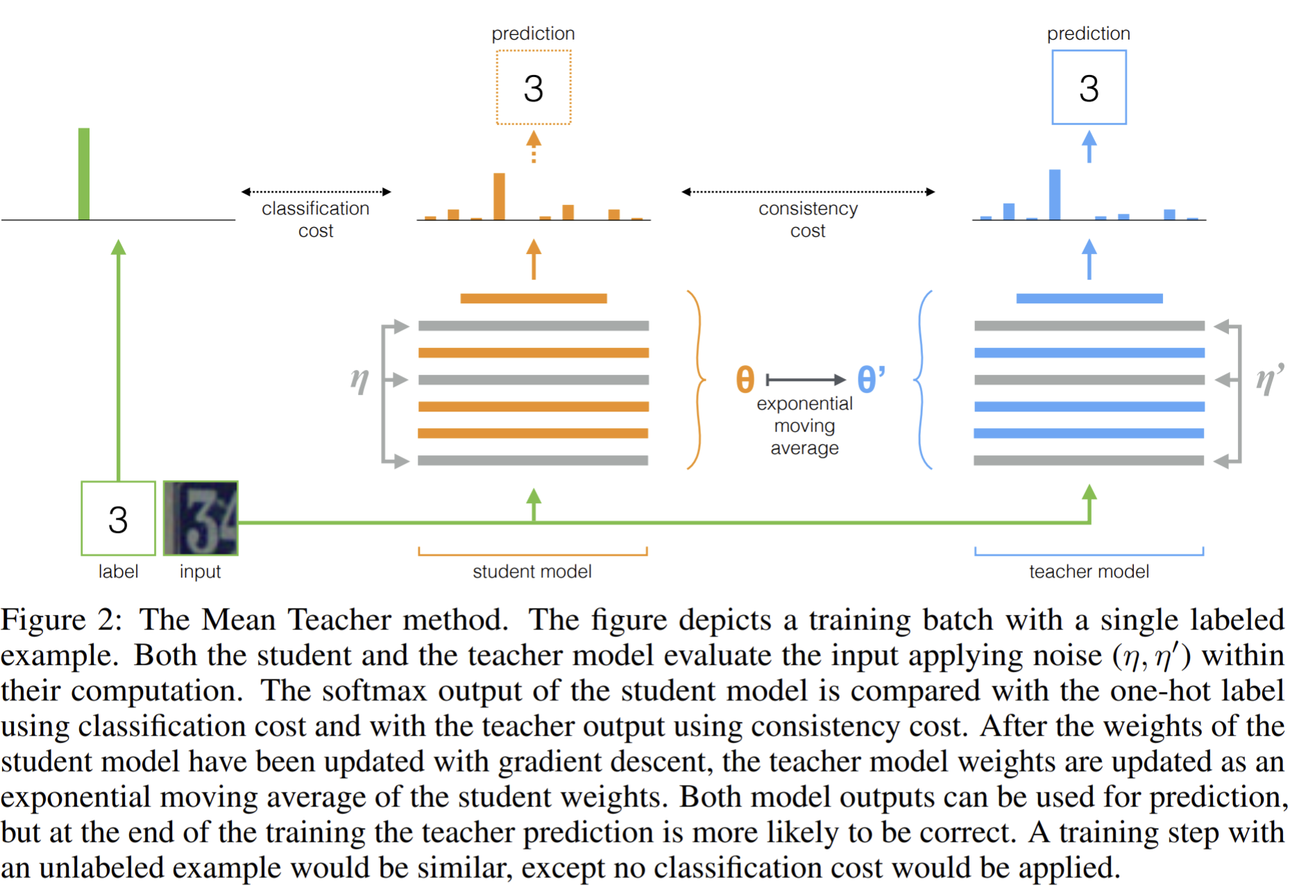
- Instead of sharing the weights with the student model, the teacher model uses the EMA weights of the student model after every step (rather than every epoch)
- Lead to weights improvement over all layers and thus the target model has better intermediate representations
- The more accurate target labels lead to a faster feedback loop between the student and the teacher models, resulting in better test accuracy
- The approach scales to large datasets and online learning
- Lead to weights improvement over all layers and thus the target model has better intermediate representations
- The loss is defined as the consistency cost between the teacher and the student:
 , where the former term is the teacher's and the latter one is the student's.
- With EMA on weights: \(\theta'_t=\alpha \theta'_{t-1}+(1-\alpha) \theta_t\). For temporal ensembling and mean teacher, the \(\theta'\) is treated as a constant with regards to optimization.
- approximate the consistency cost function \(J\) by sampling noise \(\eta,\eta'\) at each training step with stochastic gradient descent.
- use mean squared error (MSE) as the consistency cost in most of our experiments
Experiments
- Backbone: a 13-layer ConvNet.
- Augmentations/noise: random translations, horizontal flips of the input images, gaussian noise on the input layer and dropout within the network
- Benchmarks: SVNH, CIFAR-10
- Mean Teacher improves test accuracy over the \(\prod\) model and Temporal Ensembling on semi-supervised SVHN tasks. Mean Teacher also improves results on CIFAR-10 over our baseline \(\prod\) model.
- the EMA-weighted models give more accurate predictions than the bare student models after an initial period.
- Mean Teacher helps when labels are scarce.
- But in the all-labeled case (left column), Mean Teacher and the\(\prod\) model behave virtually identically.
- Either input augmentation or dropout is necessary for passable performance of our model. And input noise does not help when augmentation is in use. Dropout on the teacher side provides only a marginal benefit over just having it on the student side, at least when input augmentation is in use.
- Sensitivity to EMA decay and consistency weight.
- In each case the good values span roughly an order of magnitude and outside these ranges the performance degrades quickly.
- In the evaluation runs we used EMA decay \(\alpha\) = 0.99 during the ramp-up phase, and \(\alpha\) = 0.999 for the rest of the training. We chose this strategy because the student improves quickly early in the training, and thus the teacher should forget the old, inaccurate, student weights quickly. Later the student improvement slows, and the teacher benefits from a longer memory.
- Decoupling classification and consistency: The consistency to teacher predictions may not necessarily be a good proxy for the classification task, especially early in the training.
- To investigate, we changed the model to have two top layers and produce two outputs. . We then trained one of the outputs for classification and the other for consistency
- a moderate decoupling seems to have the benefit of making the consistency ramp-up redundant.
- Changing from MSE to KL-divergence: in this setting MSE performs better than the other cost functions.
- the results improve remarkably with the better network architecture. (ResNet)
Paper 20: Bootstrap Your Own Latent: A New Approach to Self-Supervised Learning (BYoL). ArXiv 2020
https://github.com/deepmind/deepmind-research/tree/master/byol
Previous
- SOTA contrastive methods need careful treatment of negative pairs by either relying on large batch sizes, memory Banks or customized mining strategies to retrieve the negative pairs. And their performance critically depends on the choice of image augmentation.
- Previous methods based on bootstrapping have used pseudo-labels, cluster indices or a handful of labels
- BYOL is more resilient to changes in the batch size and in the set of image augmentations compared to its contrastive counterparts.
- DeepCluster: it clusters data points using the prior representation, and uses the cluster index of each sample as a classification target for the new representation. While avoiding the use of negative pairs, this requires a costly clustering phase and specific precautions to avoid collapsing to trivial solutions.
- Hints: Predictions of Bootstrapped Latents (BPL), a SSL learning technique for RL.
- PBL jointly trains the agent’s history representation and an encoding of future observations.
- The observation encoding is used as a target to train the agent’s representation, and the agent's representation as a target to train the observation encoding.
- Hints of slow-moving average target network to produce stable targets for the online network: deep RL. But most RL methods use fixed target networks.
What
- For learning image representations. BYOL doesn't rely on negative pairs and thus is more robust the choice of image augmentations.
- Starting from an augmented view of an image, BYOL trains its online network to predict the target network’s representation of another augmented view of the same image
- We hypothesize that the combination of (i) the addition of a predictor to the online network and (ii) the use of a slow-moving average of the online parameters as the target network encourages encoding more and more information within the online projection and avoids collapsed solutions.
- Contributions
- We introduce BYOL, a SSL method which achieves state-of-the-art results under the linear evaluation protocol on ImageNet without using negative pairs.
- show that our learned representation outperforms the SOTA on semi-supervised and transfer benchmarks
- BYOL is more resilient to changes in the batch size and in the set of image augmentations compared to its contrastive counterparts.
- BYOL slightly underperforms SimCLR.
How
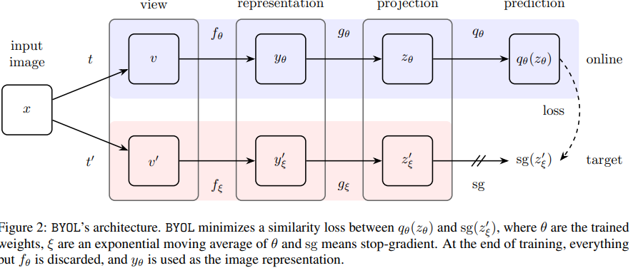
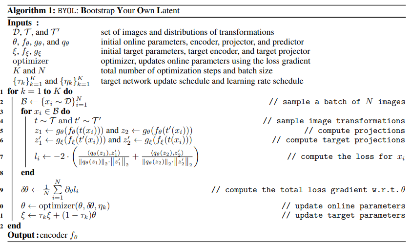
- Predicting directly in representation space can lead to collapsed representations. We thus tasked ourselves to find out whether these negative examples are indispensable to prevent collapsing while preserving high performance.
- Networks
- The online network: consists of an encoder \(f_\theta\), a projector \(g_\theta\), a predictor \(q_\theta\). The predictor is only applied on the online branch, making the architecture asymmetric between the online and target pipeline.
- The target network has the same architecture as the online one, but uses a different weight set \(\xi\).
- The target network provides the regression targets to train the online network
- The \(\xi\) are an exponential moving average of the online parameters \(\theta\). \(\xi \leftarrow \tau\xi + (1-\tau)\theta\).
- Loss:

- Term 2, the same format but denoted as \(\tilde{\mathcal{L}}_{\theta,\xi}\), by input \(v'\) into online branch, and \(v\) into target branch.
- Finally, the total loss is \(\mathcal{L}_{\theta,\xi}^{BYOL}=\mathcal{L}_{\theta,\xi}+\tilde{\mathcal{L}}_{\theta,\xi}\), with respect \(\theta\) at each training step.
- Update BYOL:

- We hypothesize that the main role of BYOL’s moving-averaged target network is to ensure the near-optimality of the predictor over training;
- if we were to minimize \(\mathbb{E}[\sum_i Var(z'_{\xi,i}|z_\theta)]\) with respect to \(\xi\), we would get a collapsed \(z'_{\xi}\) as the variance is minimized for a constant \(z'_{\xi}\).
- Augmentations: compositions of the behind image augmentations in the listed order
- random cropping
- optional left-right flip
- color jittering: color distortion, consisting of a random sequence of brightness, contrast, saturation, hue adjustments
- color dropping: an optional grayscale conversion
- gaussian blurring
- solarization
- Architecture
- the representation y corresponds to the output of the final average pooling layer, which has a feature dimension of 2048 (for a width multiplier of 1×)
- The \(g_\theta\) is a MLP consists in a linear layer with output size 4096 followed by batch normalization rectified linear units (ReLU).
- the output of this MLP is not batch normalized
- the weights of the target network represent a delayed and more stable version of the weights of the online network
- Training skills
- LARS optimizer with a cosine decay learning rate schedule, without restarts, over 1000 epochs, with a warm-up period of 10 epochs.
- set the base learning rate to 0.2, scaled linearly [72] with the batch size (LearningRate = 0.2 × BatchSize/256). In addition, we use a global weight decay parameter of 1.5 · 10−6 while excluding the biases and batch normalization parameters from both LARS adaptation and weight decay.
- The target network, the exponential moving average parameter \(\tau\) starts from \(\tau_{base} = 0.996\) and is increased to one during training.
- \(\tau\triangleq 1 − (1 − \tau_{base}) · (cos(πk/K) + 1)/2\) with \(k\) the current training step and \(K\) the maximum number of training steps.
- 4096 batch size
Experiments
- Transfer to other vision tasks: evaluate on object detection by reproducing the setup using a Faster R-CNN architecture. We fine-tune on trainval2007 and report results on test2007 using the standard AP50 metric;
- Ablation study
- Batch size: BYOL is not that sensitive as SimCLR while decreasing the batch size
- Image augmentations: Not like SimCLR, even if augmented views of a same image share the same color histogram, BYOL is still incentivized to retain additional features in its representation.<==the performance of BYOL is much less affected than the performance of SimCLR when removing color distortions from the set of image augmentations (−9.1 accuracy points for BYOL, −22.2 accuracy points for SimCLR).
- The target network:
- It helps to provide more negative samples to MoCo.
- Adding the negative pairs to BYOL’s loss without re-tuning the temperature parameter hurts its performance.
- Simply adding a target network to SimCLR already improves performance.
- Network hyperparameters:
- removing the weight decay in either BYOL or SimCLR leads to network divergence, emphasizing the need for weight regularization in the self-supervised setting.
- changing the scaling factor in the network initialization did not impact the performance
- Relation with mean teacher
- Removing the predictor in BYOL results in an unsupervised version of MT with no classification loss that uses image augmentations instead of the original architectural noise (e.g., dropout). But this operation hurts the performance
- Importance of a near-optimal predictor
- we can remove the target network without collapse by making the predictor near-optimal, either by (i) using an optimal linear predictor (obtained by linear regression on the current batch) before back-propagating the error through the network (52.5% top-1 accuracy), or (ii) increasing the learning rate of the predictor
- keeping the predictor near-optimal at all times is important to preventing collapse, which may be one of the roles of BYOL's target network.
- One notable exception is RMS error for NYU Depth prediction, which is a metric that’s sensitive to outliers. The reason for this is unclear, but one possibility is that the network is producing higher-variance predictions due to being more confident about a test-set scene’s similarities with those in the training set.
- The predictor learning rate needs to be higher than the projector learning rate in order to successfully remove the target network. This further suggests that the learning dynamic of predictor is central to BYOL’s stability.
Paper 21: Understanding self-supervised and contrastive learning with "Bootstrap Your Own Latent" (BYOL) Blog post
https://github.com/untitled-ai/self_supervised
Findings:
(1) BYOL often performs no better than random when batch normalization is removed, and
(2) the presence of batch normalization implicitly causes a form of contrastive learning.
it appears that the primary reason BYOL works is that it is doing a form of contrastive learning—just via an indirect mechanism.
BYOL builds on the momentum network concept of MoCo, adding an MLP \(q_\theta\)to predict \(z'\) from \(z\).
We found the BN in MLP head is important in BYOL, while MoCo does not care the existence of BN.==> view BN as a new way to implement contrastive learning on embedded representations.
- the activations of other inputs in the same mini-batch are essential in helping BYOL find useful representations.
- The function \(q\) cannot learn the identity function if the mini-batch inputs are very similar: the batch normalization will redistribute the activations through vector space so that the final layer predictions are all very different.
- One way to prevent mode collapse is to identify the common mode between examples. BN identifies this common mode between examples of a mini-batch and removes it by using the other representations in the mini-batch as implicit negative examples.
- with batch normalization, BYOL learns by asking, "how is this image different from the average image?"
We measured the average cosine similarity between the projections of positive examples (in blue), as well as the similarity to the projections from negative examples from the same mini-batch (in red) over each mini-batch in the tenth epoch of training.
Earlier batch normalization layers have the same effect (eventually)
Removing all batch normalization completely prevents learning—unless at least one technique is used to prevent mode collapse.
Paper 22: Data-Efficient Reinforcement Learning with Momentum Predictive Representations. ArXiv 2020
https://github.com/mila-iqia/spr
Previous
- Learning from limited interaction remains a key challenge
- collecting interaction data for many real-world tasks is costly, making improved data efficiency a prerequisite for successful use of deep RL in these settings
- Deep Q-learning for DQN
- Distributional RL models the full distribution of future reward rather than just the mean
- Dueling DQN: decouple the \(value\) of a state from the advantage of taking a given action in that state.
- Double DQN: modifies the Q-learning update to avoid overestimation due to the \(\max\) operation.
- Rainbow: consolidates these improvements into a single combined algorithm and has been adapted to work well in data-limited regimes
- Representation learning in RL
- CURL: a combination of image augmentation and a contrastive loss to perform representation learning for RL. But most of the benefits of CURL come from image augmentation
- CPC, CPC|Action, ST-DIM, DRIML: optimize various temporal contrastive losses in reinforcement learning.
- DeepMDP: similar as SPR, but it uses online encoder to generate prediction targets.
- PBL: directly predicts representations of future states but it uses two separate target networks trained via gradient descent. And it studies multi-task generalization in the asymptotic limits of data.
What
- posit that an agent can learn more efficiently if we augment reward maximization with self-supervised objectives based on structure in its visual input and sequential interaction with the environment
- Self-Predictive Representations (SPR), trains an agent to predict its own latent state representations multiple steps into the future, which is an encoder by exponential moving average of the agent’s parameters.
- The full self-supervised objective combines future prediction and data augmentation, where the data augmentation loss forces the agent’s representations to be consistent across multiple views of an observation. Note the data augmentation is also applied on the future prediction task.
- train better state representations for RL by forcing representations to be temporally predictive and consistent when subject to data augmentation.
How
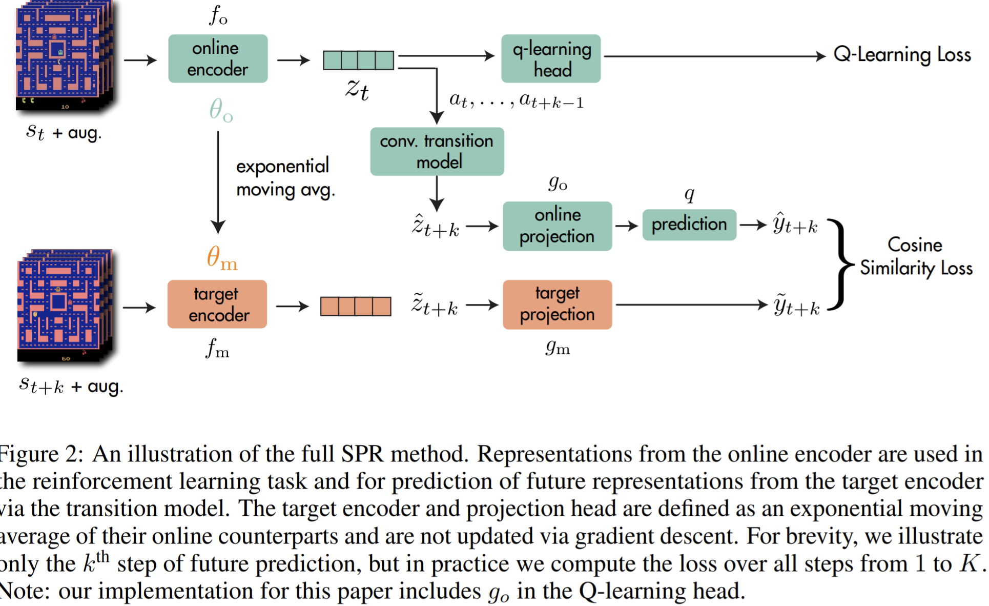
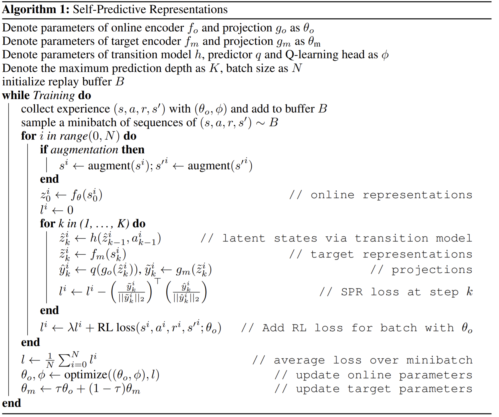
seek to train an agent whose expected cumulative reward in each episode is maximized
Deep Q learning
- Deep Q Networks trains a neural network \(Q_\theta\) to approximate the agent’s current Q-function (policy evaluation) while updating the agent’s policy greedily with respect to this Q-function (policy improvement).
- Loss: minimize the error between predictions from \(Q_\theta\) and a target value estimated by \(Q_\xi\) (an earlier version of the network), $_{}{DQN}=(Q_(s_t,a_t)-(r_t+Q(s_{t+1},a)))2 $
Self-predictive representations: set the maximum number of steps into the future which we want to predict as \(K\).
Online and target networks
- Online encoder \(f_o\) to transform observed states \(s_t\) into representations $z_tf_o(s_t) $.
- augment each observation \(s_t\) independently when using data augmentation.
- computing target representations for future states using a target encoder \(f_m\), whose parameters are an exponential moving average (EMA) of the online encoder parameters. \(\theta_m\leftarrow \tau \theta_m+(1-\tau)\theta_o\).
- When \(\tau=0,\theta_m=\theta_o\) performs well when regularization is already provided by data augmentation.
transition model: and prediction loss operate in the latent space, thus avoiding pixel-based reconstruction objectives.
- compute \(\hat{z}_{t+1:t+K}\) iteratively: \(\hat{z}_{t+k+1}\triangleq h(\hat{z}_{t+k, a_{t+k}})\), starting from \(\hat{z}_t \triangleq z_t \triangleq f_o(s_t)\).
- \(\tilde{z}_{t+k}\triangleq f_m(s_{t+k})\).
projection heads: use online and target projection heads \(g_o,g_m\), and another prediction head \(q\).
- \(\hat{y}_{t+k}\triangleq q(g_o(\hat{z}_{t+k})),\forall \hat{z}_{t+k}\in \hat{z}_{t+1:t+K}\)
- \(\tilde{y}_{t+k}\triangleq g_m(\tilde{z}_{t+k}),\forall \tilde{z}_{t+k}\in \tilde{z}_{t+1:t+K}\).
- \(g_m\)'s parameters are updated by an EMA of the \(g_o\).
prediction loss: the future prediction loss for SPR by summing over cosine similarities between the predicted and observed representations at timesteps \(t+k\) for \(1\leq k\leq K\):

Optimization
- SPR loss affects \(f_o,g_o,q,h\)
- Q-learning loss affects \(f_o\) and the Q-learning head.
- Full loss \(\mathcal{L}_\theta^{total}=\mathcal{L}_\theta^{RL}+\lambda \mathcal{L}_\theta^{SPR}\).
Transition model architecture
- \(h\): CNN to the 64 × 7 × 7 spatial output of the convolutional encoder \(f_o\).
- one-hot vector for representing the action.
- The maximum prediction depth is 5.
Data augmentations
- small random shifts and color jitter
- normalize activations to lie in \([0, 1]\).
If without augmentation, find that SPR performs better when dropout with probability \(0.5\) at each layer in the online and target encoders. Also adding noise if without image-specific augmentations.
Experiments
- 3-layer CNN encoder and 10-step returns for Q-learning
- We show that data augmentation can be more effectively leveraged in reinforcement learning by forcing representations to be consistent between different augmented views of an observation while also predicting future latent states.
- Measurements
- evaluate the performance of different methods by computing the average episodic return at the end of training.
- Human-normalized score: \(\frac{agent score-randomscore}{humanscore-randomscore}\) and aggregated across the 26 games by mean or median.
- self-normalized score: \(\frac{agent score-randomscore}{averagescore-randomscore}\).
- normalize scores with respect to expert human scores
- Report DQN-normalized scores,
- evaluate the performance of different methods by computing the average episodic return at the end of training.
- Analysis
- A separate target encoder is vital in all cases.
- The success of τ = 0 is interesting, since the related method BYOL reports very poor representation learning performance in this case.==> They explain that optimizing a reinforcement learning objective is in parallel with the SPR loss, since it provides an addition gradient which discourages representational collapse.
- Dynamic modeling is a key: extended dynamics modeling consistently improves performance up to roughly K = 5.
- Comparison with contrastive loss: SPR consistently outperforms both temporal and non-temporal variants of contrastive losses, including CURL.
- Using a quadratic loss causes collapse: SPR uses a cosine similarity objective which will set it in contrast to some previous works. If minimizes un-normalized L2 loss (Quadratic SPR), the model collapse.
- Projection are critical: Two possible explanations: Employing the first layer of the DQN head as a projection thus allows the SPR objective to affect far more of the network, while in this variant its impact is limited; Second, the effects of SPR in forcing invariance to augmentation may be undesirable at this level.
- A separate target encoder is vital in all cases.
Paper 23: Born Again Neural Networks. NeurIPS 2017
Previous
- Although the student cannot match the teacher when trained directly on the data, the distillation process brings the student closer to matching the predictive power of the teacher.
- KD
- Ba & Caruana (2014) demonstrated a method to increase the accuracy of shallow neural networks, by training them to mimic deep neural networks, using an penalizing the L2 norm of the difference between the student’s and teacher’s logits.
- Romero et al. (2014) aim to compress models by approximating the mappings between teacher and student hidden layers, using linear projection layers to train the relatively narrower students.
- dark knowledge: a student model trains with the objective of matching the full softmax distribution of the teacher model.
- compresses the learned function into shallow multilayer perceptrons containing 1, 2, 3, 4, and 5 layers
- force the student to match the attention map of the teacher at the end of each residual stage
- minimize the difference between teacher and student derivatives of the loss with respect to the input
- Key differences
What
- the first, to our knowledge, to demonstrate that dark knowledge, applied for self-distillation, even without softening the logits results in significant boosts in performance
- train students parameterized identically to their teachers.
- explore two distillation objectives: (i) Confidence-Weighted by Teacher Max (CWTM) and (ii) Dark Knowledge with Permuted Predictions (DKPP)
- revisit KD with the objective of disentangling the benefits of this training technique from its use in model compression
- we develop a simple re-training procedure: after the teacher model converges, we initialize a new student and train it with the dual goals of predicting the correct labels and matching the output distribution of the teacher. This is named as born-again networks (BANs)
- BANs consistently have lower validation errors than their teachers
- KD can be decomposed into two terms: a dark knowledge term, containing the information on the wrong outputs, and a ground-truth component which corresponds to a simple rescaling of the original gradient that would be obtained using the real labels.
- we demonstrate that weak masters can still improve performance of students, and KD need not be used with strong masters
How
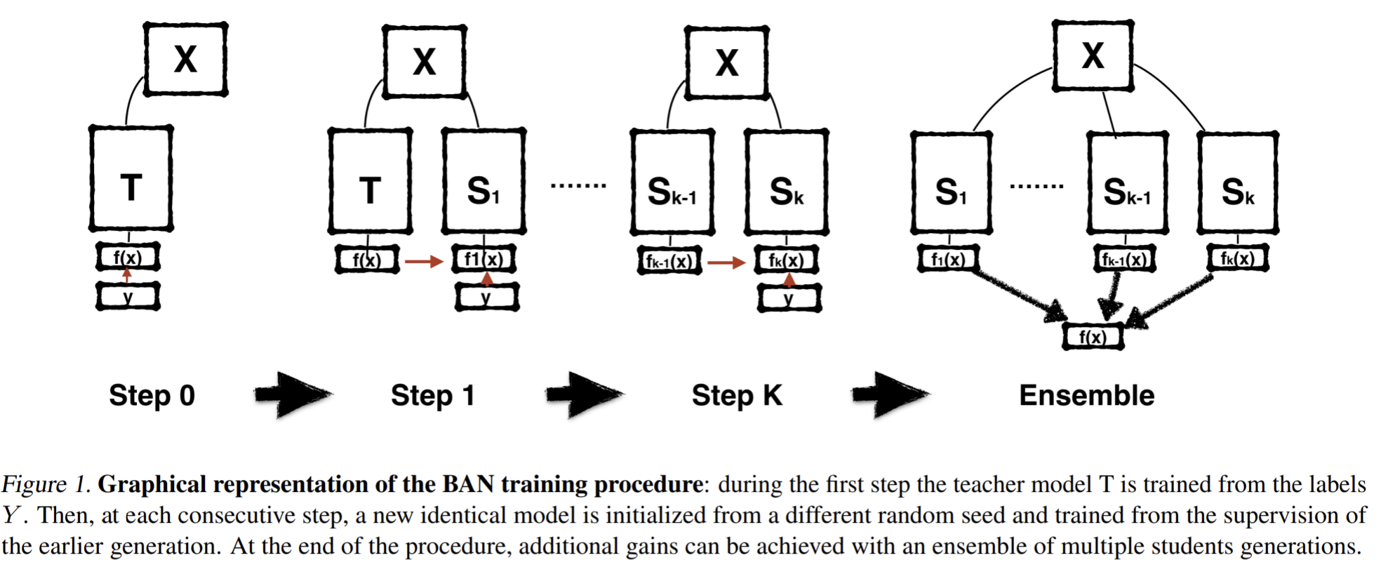
The teacher and student has the same architecture
The sequence of teaching selves born-again networks ensemble
- we apply BANs sequentially with multiple generations of knowledge transfer. In each case, the \(k\)-th model is trained, with knowledge transferred from the \(k − 1\)-th student:

- Then, we produce Born-Again Network Ensembles (BANE) by averaging the prediction of multiple generations of BANs: \(\hat{f}^k(x) =\sum_{i=1}^k f(x,\theta_i)/k\).
- we apply BANs sequentially with multiple generations of knowledge transfer. In each case, the \(k\)-th model is trained, with knowledge transferred from the \(k − 1\)-th student:
dark knowledge under the light
- When the loss is computed with respect to the complete teacher output, the student back-propagates the mean of the gradients with respect to correct and incorrect outputs across all the \(b\) samples \(s\) of the mini-batch:

- The second term corresponds to the information incoming from all the wrong outputs.
- The first term corresponds to the gradient from the correct choice and allows the interpretation of the output of the teacher \(p^*\) as a weighting factor of the original ground truth label \(y^*\).
- When the loss is computed with respect to the complete teacher output, the student back-propagates the mean of the gradients with respect to correct and incorrect outputs across all the \(b\) samples \(s\) of the mini-batch:
does the success of dark knowledge owe to the information contained in the nonargmax outputs of the teacher? Or is dark knowledge simply performing a kind of importance weighting?
In the first treatment, Confidence Weighted by Teacher Max (CWTM), we weight each example in the student’s loss function (standard cross-entropy with ground truth labels) by the confidence of the teacher model on that example. This means they will take the correct answer \(p_{∗,s}\) with the max output of the teacher \(\max p_{.,s}\).

dark knowledge with Permuted Predictions (DKPP), we permute the non-argmax outputs of the teacher’s predicted distribution.
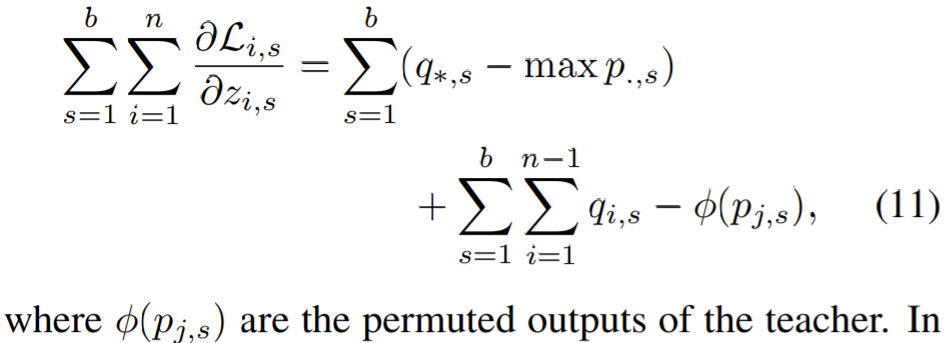
Experiments
- Benckmark: CIFAR-100
Plans
- we construct Wide-ResNet and bottleneck-ResNet networks that match the output shape of DenseNet-90-60 at each block, as baselines for our BAN-ResNet with DenseNet teacher experiment.
- Strategies of knowledge transfer for training BANs
- progressively constraining the BANs to be more similar to their teachers, sharing the first and last layers between student and teacher
- adding losses that penalize the L2 distance between student and teacher activations
- simple KD via cross entropy: performs the best.
- BAN without dark knowledge
- CWTM: interpret the max of the teacher’s output for each sample as the importance weight and use it to rescale each sample of the student’s loss.
- DKPP: maintain the overall high order moments of the teachers output, but randomly permute each output dimension except the argmax one.
- Apply on Penn Tree Bank dataset to test if the model can work on NLP domain beyond cv domain.
Results
- our largest ensemble BAN-3- DenseNet-BC-80-120 with 150M parameters and an error of 14.9% is the lowest reported ensemble result in the same setting. But the teacher is used as one of the ensemble for final inference.
- Importance weights CWTM lead to weak improvements over the teacher in all models but the largest DenseNet.
- The information contained in pre-trained models can be used to rebalance the training set, by giving less weight to training samples for which the teacher’s output distribution is not concentrated on the max.
- DenseNet students are particularly robust to the variations in the number of layers
- Smaller reductions lead to larger parameter savings with lower accuracy losses, but directly choosing a smaller network retrained with BAN procedure like DenseNet-106-33 seems to lead to higher parameter efficiency.
- our Wide-ResNet and Pre-ResNet students that match the output shapes at each stage of their DenseNet teachers tend to outperform classical ResNets, their teachers, and their baseline.
- LSTM models work only when trained with a combination of teacher outputs and label loss (BAN+L).
Paper 24: Training Deep Neural Networks in Generations: A More Tolerant Teacher Educates Better Students. AAAI 2019
Previous
- Existing approaches mostly used a hard distribution (e.g., one-hot vectors) in training, leading to a strict teacher which itself has a high accuracy
- We argue that the teacher needs to be more tolerant, although this often implies a lower accuracy.
- But this is not necessarily the optimal target to fit, because except for maximizing the confidence score of the primary class (i.e., the ground-truth), allowing for some secondary classes (i.e., those visually similar ones to the ground-truth) to be preserved may help to alleviate the risk of over-fitting
- deal with per-image similarity, one way is teacher-student optimization
- using various ways of supervision,
- using multiple teachers to provide a better guidance,
- adding supervision in intermediate neural responses,
- and allowing two networks to help optimize each other
- Born again networks: optimize the same network in generations, in which the next generation was guided by two terms, namely, the standard cross-entropy loss and the KL-divergence between the teacher and student signals. The students are supervised by both the truth labels and predicted labels from teachers.
What
- Training a deep neural network in generations
- Build tolerant teacher by merely an extra loss term added to the teacher network, facilitating a few secondary classes to emerge and complement to the primary class. This provides milder supervision signal and make students to learn from inter-class similarity and potentially lower the risk of overfitting.
- The teacher and the student have the same architecture.
How
- Traditional teacher-student model
- teacher \(f(x_n,\theta)\): trained by

- student \(f(x_n,\theta^S)\):

- The teacher provides one-hot vector \(\mathrm{y}_n\).
- teacher \(f(x_n,\theta)\): trained by
- We find that a deep network is able to automatically learn semantically similar classes for each image individually1 . We name it as secondary information, which corresponds to the primary information provided by supervision.
- (After analyzing the confidence score by born-again process with 110-later ResNet on CIFAR100)
- the student network can avoid being fit to unnecessarily strict distributions and thus generalizes better
- Towards High-Quality Secondary Information:
- three ways to achieve: the first two push the score distribution (after softmax) towards less peaked at the primary class, but have a drawback that they facilitate the confidence scores to distribute over all classes, regardless if these classes are visually similar to the training sample.
- LSR (label smoothing regularization ): the added term is the KL-divergence between the score distribution and the uniform distribution
- CP (confidence penalty): the negative entropy gain
- the way this papers authors do: pick up a few classes which have been assigned with the highest confidence scores, and assume that these classes are more likely to be semantically similar to the input image.
- the way this papers authors do:
- set a fixed integer \(K\) which stands for the number of semantically reasonable classes for each image, including the primary class.
- TSD (top score difference ): compute the gap between the confidence scores of the primary class and other \(K-1\) classes with highest scores:
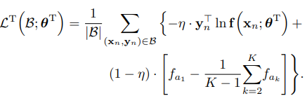 , were \(f_{ak}^{\mathrm{T}}\) is short for the \(k\)-th largest element of \(f(x_n,\theta^{\mathrm{T}})\).
- To summary: LSR features are much more discriminative (both \(Dist^C, Dist^S\) are much larger, CP is similar).
- three ways to achieve: the first two push the score distribution (after softmax) towards less peaked at the primary class, but have a drawback that they facilitate the confidence scores to distribute over all classes, regardless if these classes are visually similar to the training sample.
- To test
- These 100 classes are partitioned into 20 superclasses, with 5 fine-level classes in each superclass \(S_j\) . We compute the mean vector for each class, denoted by \(v^C_i , i = 1, 2, \cdots , 100\), and for each superclass, denoted by \(v^S_j , j = 1, 2, \cdots, 20\), respectively.
- Two statistics: increasing \(Dist^S\) so that coarse-level classification becomes better, meanwhile decreasing \(Dist^C\) so that reasonable secondary information is preserved and learned by students.
- measures how much feature vector \(v^C_i\) differs from the mean of its superclass, \(v^S_j\) where \(i\in S_j\).

- measures the difference between each \(v^S_j\) and the overall average vector \(v^A = \frac{1}{20} v^S_j\).

- The best classification accuracy is obtained by TSD-0.6, where \(u(\eta)\) is an intuitive way of parameterizing \(\eta\), with a parameter not too high or low. ==> in teacher-student optimization, the student learns best from a teacher that preserves reasonable secondary information.
- measures how much feature vector \(v^C_i\) differs from the mean of its superclass, \(v^S_j\) where \(i\in S_j\).
- Details of Training in Generations
- \(u(\eta)\)
- \(f_{a1}^T\doteq u(\eta) = \min \{\frac{\eta}{1-\eta}\cdot \frac{K-1}{K},1\}\), which is monotonically increasing with respect to \(\eta\).==> optimize on $u() $ is equal to optimize on \(\eta\).
- a deeper network often requires a larger u(η), or equivalently a larger η, in order to get better trained.
- In practice, we fix \(K = 5\) for simplicity.
- the entire optimization process is parameterized by \(K, η,\lambda\)
- the secondary information in teacher signals is gradually weakened, and recognition accuracy may saturate and start to descend after a few generations.
- \(u(\eta)\)
Experiments
- Benchmark: CIFAR100, ILSVRC2012
- Bacbone: Resnet 20, 56, 110, DenseNets 100, 190.
- recognition accuracy often saturates after a few generations, because eventually the teacher signal will converge to the points that are dominated by the primary classes and the teacher will become strict again. The saturated accuracy is still much higher than the baseline.
- In DenseNet-190, our results are competitive among the state-of-the-arts.
- Test on ILSVRC2012
- use D(0.6, 0.6), as the basic network (18 layers) is not very deep).
- K = 5, u (η) = 0.6 and λ = 0.6.
- Similar behaviors of the scores: start with a worse patriarch6 , enjoy gradual and persistent improvement from generation to generation, and achieve saturation after several generations.
Paper 25: Variational information distillation for knowledge transfer. CVPR 2019
Previous
- Existing knowledge transfer approaches match the activations or the corresponding handcrafted features of the teacher and the student networks.
- KD
- match the final layers of the teacher and the student network, as the outputs from the final layer of the teacher network provide more information than raw labels
- match intermediate layers of the student network to the corresponding layers of the teacher network
- recently: relax the regularization of matching the entire layer by matching carefully designed features/statistics extracted from intermediate layers of the teacher and the student networks, e.g., attention maps and maximum discrepancy.
- there is no commonly agreed theory behind knowledge transfer
What
- knowledge transfer across heterogeneous network architectures by transferring knowledge from a convolutional neural network (CNN) to a multi-layer perceptron (MLP) on CIFAR-10.
- information-theoretic framework for knowledge transfer which formulates knowledge transfer as maximizing the mutual information between the teacher and the student networks, named as variational information distillation (VID).
- Use variational information maximization considering the mutual information is not tractable
- existing knowledge transfer methods (two are listed in their paper) can be derived as specific implementations of our framework by choosing different forms of the variational lower bound
How
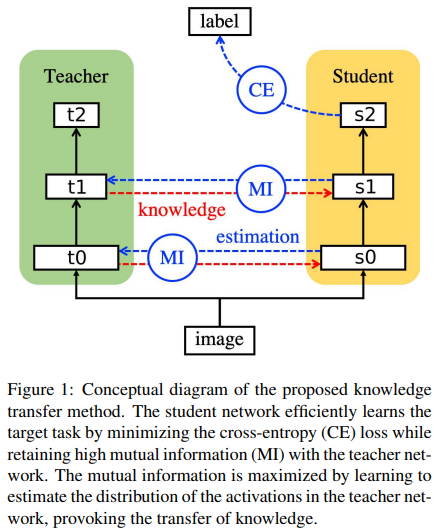
VID
- consider an input random variable \(x\) drawn from the target data distribution $p(x) $ and \(K\) pairs of layers \(\mathcal{R} = \{(\mathcal{T} (k) , \mathcal{S} (k) )\}^K_{k=1}\) where \((\mathcal{T} (k) , \mathcal{S} (k))\) are sampled from the teacher and student respectively
- The mutual information between the pair of random variables \((t, s)\) is defined by:
 , which can be understood as a reduction in uncertainty in the knowledge of the teacher encoded in its layer \(t\) when the student layer \(s\) is known.
 - Simply, the loss is
 , with \(\mathcal{L}_S\) the task-specific loss function for the target task and \(\lambda_k\) a hyper-parameter introduced for regularization of the mutual information in each layer.
 - Since the exact mutual information is hard to be tracked, they use VID to get \(I(t;s)\geq H(t) + \mathbb{E}_{t,s}[\log q(t|s)]\).
- Then the final loss is simplified as
 , where \(H(t)\) is removed since the constancy. It helps jointly train the student network for the target task and maximization of the conditional likelihood to fit the activations of the selected layers from the teacher network.
Choice of variational distribution \(q(t|s)\)
 , where \(\sigma^2_c =\log (1+\exp(\alpha_c))+\epsilon\) for numerical stability.
If layer \(t=\mathcal{T}^{(logit)}(x)\), aka the layer t corresponds to the Logitech layer of the teacher network, then

where \(t_n\) is the \(n\)-th entry of the vector \(t\), \(\mu_n\) represents the output of a single unit of NN and \(\sigma_n\) is, again, parameterized by softplus function to enforce positivity. And the corresponding layer \(s\) is the penultimate layer instead of the logit layer to match the hierarchy of two layers without being too restrictive on the output of the student network.
we found that using a simple linear transformation for the parameterization of the mean function was sufficient in practice. \(\mu(s) =Ws\).
the parts that correspond to the background achieve higher magnitudes compared to that of the foreground in general. Our explanation is that the output of layers corresponding to the background that mostly corresponds to zero activations and contains less information, being a relatively easier target for maximizing the log-likelihood of the variational distribution.
Connections to existing works
- The infomax principle
- layers of the teacher network contain important information for the target task, and a good representation of the student network is likely to retain much of their information.
- When \(t^{(k)}=x\), the formula becomes a traditional semi-supervised learning infomax principle.
- Generalizing mean squared error matching: existing KD with MSE can be seen as a specific instance of the proposed framework, all use Gaussian distribution as the variational distribution
- The basic formula: In general, the methods will be induced from the equation (4) by making a specific choice of the layers \(\mathcal{R} = \{(\mathcal{T} (k) , \mathcal{S} (k) )\}^K_{k=1}\) for knowledge transfer and parameterization of heteroscedastic mean µ(·) in the variational distribution:

- Method matching the output of logit layers \(\mathcal{T}^{(logit) }\) , \(\mathcal{S}^{(logit) }\) from the teacher and the student networks with respect MSE: based on the basic formula, let $ = {(^{(logit)} , ^{(logit)})}, µ(s) = s $ .
- If method add a linear layer on top of the penultimate layer \(\mathcal{S}^{(pen)}\) in the student network to match the logit layer of the teacher: based on the basic formula, let $ = {(^{(logit)} , ^{(pen)} )} , µ(s) = Ws $.
- If method minimize the mean squared error between intermediate layers from the teacher and the student networks, with additional convolutional layer introduced for adapting different dimension size between each pair of matched layers: based on the basic formula, choose layers for the KD to be intermediate layers of the teacher and the student networks, and µ(·) being a linear transformation corresponding to a single 1 × 1 convolutional layer
- The basic formula: In general, the methods will be induced from the equation (4) by making a specific choice of the layers \(\mathcal{R} = \{(\mathcal{T} (k) , \mathcal{S} (k) )\}^K_{k=1}\) for knowledge transfer and parameterization of heteroscedastic mean µ(·) in the variational distribution:
- Our methods differ with the MSE KD in
- allowing the use of a more flexible nonlinear functions for heteroscedastic mean and
- modeling different variances for each dimension in the variational distribution.
- modeling unit variance for all dimensions of the layer t in the teacher network could be highly restrictive for the student network.
- Comparison with feature matching
- Previous: match attentions maps; match the maximum mean discrepancy; match the features called the Flow of Solution Procedure (FSP) defined by the Gram matrix of layers adjacent in the same network; matching the reconstructed input image from the intermediate layers of the teacher and the student networks; ==> avoiding the aforementioned over-regularization issue by filtering out information in the teacher network using expert knowledge.
- But methods in previous potentially lead to suboptimal results when the feature extraction is not apt for the particular KD task and may discard important information from the layer of the teacher network in an inversible way.
- The infomax principle
Experiments
- apply VID to two different locations: (a) VID between intermediate layers of the teacher and the student network (VID-I) and (b) VID between the logit layer of the teacher network and the penultimate layer of the student network (VID-LP).
- Also compare with other KD methods: the original knowledge distillation (KD), learning without forgetting (LwF), hint based transfer (FitNet), activationbased attention transfer (AT) and polynomial kernel-based neural selectivity transfer (NST)
- Observe: whether we can benefit from knowledge transfer in the small data regime and how much performance we lose by reducing the size of the student network?
- Reducing training data
- Use WRN (wide residual network ) as the backbone for our methods, WRN-40-2 for the teacher and WRN-16-1 for the student
- the teacher network is pre-trained on the whole training set of CIFAR-10
- KD is applied to 4 different sizes of training set, 5000(full ), 1000,500,100 data points per class.
- The performance gap increases as the size of dataset get smaller, e.g., VID-I only drops 10.26% of accuracy even when 100 data points per each class are provided to the student network.
- Varying the size of the student network
- A student network with four choices of size, i.e., WRN-40- 2, WRN-16-2, WRN-40-1, WRN-16-1, is trained on the whole training set of CIFAR-100
- when the structure of the student network is identical to that of the teacher network, i.e., WRN-40-2, two methods can be combined to yield the best performance
- Reducing training data
- Transfer learning
- Benchmarks: CUB200-2011 (bird species classification ), MIT-67 (indoor scene classification )
- Backbone: teacher ResNet-34, students ResNet 18 or VGG 9.
- ResNet-18: choose the outputs of the third and fourth groups of residual blocks (from the input) as the intermediate layers for knowledge transfer.
- VGG-9: choose the fourth and fifth max-pooling layers as the intermediate layers for knowledge transfer. This make sure students in different architecture have the same spatial dimension as the intermediate layers selected from the teacher network.
- The knowledge transfer from ResNet-34 to VGG-9 gives very similar performance to the transfer from ResNet-34 to ResNet-18 for all the knowledge transfer methods.==> knowledge transfer methods are robust against small architecture changes.
- Knowledge transfer from CNN to MLP: whether a knowledge transfer method can work between two completely different network architectures?
- Benchmark: CIFAR10
- Student: MLP with 5 FC layers, each layer has a non-linearity activation function.
- Teacher: WRN-40-2
- The knowledge transfer between intermediate layers is defined between the outputs of four residual groups of the teacher network and the outputs of the first four fully connected layers of the student network.
- our method bridges the performance gap between CNN (84.6% using one convolutional layer [27]) and MLP shown in previous works.==> KT can work between two completely different architectures.
Paper 26: Be Your Own Teacher: Improve the Performance of Convolutional Neural Networks via Self Distillation ICCV 2019
https://github.com/ArchipLab-LinfengZhang/
Previous
- boost accuracy through either deeper or wider network structures, which brings with them the exponential increment of the computational and storage cost, delaying the responding time
- Traditional KD forces student neural networks to approximate the softmax layer outputs of pre-trained teacher neural networks,
- A distinguished student model which outperforms its teacher model remains rare
- Distillation frameworks require substantial efforts and experiments to find the best architecture of teacher models, which takes a relatively long time.
- KD methods
- FitNet: reducing the distance between feature maps of students and teachers
- AT: align the features of attention regions
- some researchers extended knowledge distillation to generative adversarial problem
- KD usages:
- Absorb the students into the teacher to obtain the better generalization ability on test data.
- Use KD for data augmentation, increasing the numerical value of labels to higher entropy
- regard KD as a tool to defend adversarial attack.
- Adaptive Computation: selectively skip several computation procedures to remove redundancy. Usually focus on layers, channels and images
- Skipping some layers in neural networks: layer-wise dropout; layer-wise dropout + additional controllable modules or gating function; design early-exiting prediction branches to reduce the average execution depth in inference
- Skipping some channels in neural networks: switchable BN to dynamically adjust the channels in inference
- Skipping less important pixels of the current input images: critical details of input data; RL+DL to identify the importance of pixels in the input images before feeding into CNNs.
- Deep supervision: classifiers trained on highly discriminating features can improve the performance in inference
- additional supervision is added to train the hidden layers directly: tasks like image classification, objection detection, and medical images segmentation
- The main difference in self distillation is that shallow classifiers are trained via distillation instead of only labels ==> performance improvement
What
- propose a general training framework named self distillation, which enhances the performance (accuracy) of CNNs through shrinking the size of the network.
- self distillation framework distills knowledge within network itself: the knowledge in the deeper portion of the networks is squeezed into the shallow ones.
- The proposed self distillation not only requires less training time (from 26.98 hours to 5.87 hours on CIFAR100, a 4.6X time training shorten time), but also can accomplish much higher accuracy (from 79.33% in traditional distillation to 81.04% on ResNet50)
How
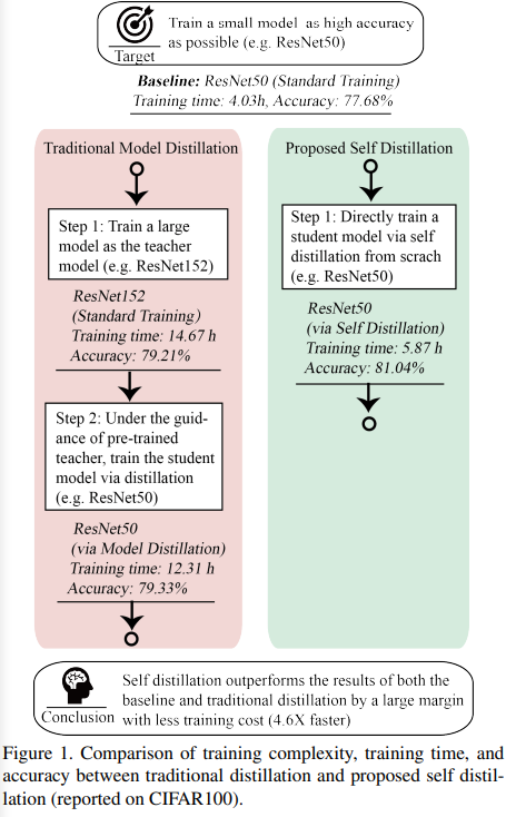
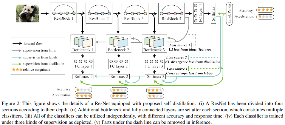
- three kinds of losses are introduced during training processes:
- Cross entropy loss from labels: to not only the deepest classifier but also all the shallow classifiers. In this way, the knowledge hidden in the dataset is introduced directly from labels to all the classifiers
- KL-divergence loss under teachers guidance: using softmax outputs between students and teachers, and introduced to the softmax layer of each shallow classifier
- L2 loss from hints: L2 loss between features maps of the deepest classifier and each shallow classifier. The inexplicit knowledge in feature maps is introduced to each shallow classifier’s bottleneck layer.
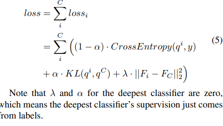
Experiments
- Benchmark: CIFAR100, ImageNet
- Backbones: ResNet, WideResNet, Pyramid ResNet, ResNeXt, VGG
- Comparison with SOTA
- With Standard training:
- The deeper the backbone neural networks are, the more improvement on performance they acquire
- naive ensemble works effectively on CIFAR100 yet with less and sometimes negative influence on ImageNet, which may be caused by the larger accuracy drop in shallow classifiers, compared with that on CIFAR100
- Classifiers’ depth plays a more crucial part in ImageNet, indicating there is less redundancy in neural networks for a complex task.
- with Distillation
- All the performance of distillation methods outperforms the directly trained student networks.
- Although self distillation doesn’t have an extra teacher, it still outperforms most of the rest distillation methods
- with Deeply Supervised Net
- Self distillation outperforms deep supervision in every classifier.
- Shallow classifiers benefit more from self distillation.==> Better shallow classifiers can obtain more discriminating features, which enhances the deeper classifiers performance in return.
- With Standard training:
- Scalable Depth for Adapting Inference
- Ensemble of the deepest three classifiers can bring 0.67% accuracy improvement on average level with only 0.05% penalty for computation, owing to that different classifiers share one backbone network
- Other discussion
- Self distillation can help models converge to flat minima which features in generalization inherently
- Keskar et al. proposed explanations that over-parameters models may converge easier to the flat minima, while shallow neural networks are more likely to be caught in the sharp minima, which is sensitive to the bias of data
- the proposed self distillation framework can converge to a flat minimum.
- as standard deviation of the Gaussian noises, keeping increasing, while the training accuracy in the model without self distillation drops severely
- the models trained with self distillation are more flat==> the model trained without self distillation is much more sensitive to the Gaussian noise. These experiments results support our view that self distillation helps models find flat minima.
- Self distillation prevents models from vanishing gradient problem
- compute the mean magnitude of gradients in each convolutional layer. Two 18-layer ResNets are trained, one of them equipped with self distillation and the other not.
- gradients of the model with self distillation is larger than the one without self distillation, especially in the first and second ResBlocks.
- More discriminating features are extracted with deeper classifiers in self distillation
- the deeper the classifier is, the more concentrated clusters are observed.
- the changes of the distances in shallow classifiers, are more severe than that in deep classifiers.
- the more discriminating feature maps in the classifier, the higher accuracy the model achieves.
- Unexplored future works
- Automatic adjustment of newly introduced hyper-parameters
- Is the flat minimum found by self distillation ideal?
- Self distillation can help models converge to flat minima which features in generalization inherently
Paper 27: Müller et al (2019) When Does Label Smoothing Help? NeurIPS 2019
Previous
- soft targets that are a weighted average of the hard targets and the uniform distribution over labels, and generalize well: may relate to information bottleneck theory that explains generalization in terms of compression.
- label smoothing is still poorly understood
- Pereyra et al.: label smoothing is equivalent to confidence penalty if the order of the KL divergence between uniform distributions and model’s outputs is reversed. Unigram label smoothing if the output labels' distribution is not balanced.
- label dropout, whereas label smoothing is the marginalized version of label dropout.
- Calibration of sequence models
- investigate the sequence level calibration of machine translation models and conclude they are remarkably well calibrated.
- calibration of next-token prediction in language translation: calibration of SOTA can be improved by a parametric model
- neither work invesigates the relation between label smoothing during training and calibration
- Some check the effect of softmax temperature and label smoothing on decoding accuracy
What
- In addition to improving generalization, label smoothing improves model calibration which can significantly improve beam-search, so that the confidences of their predictions are more aligned with the accuracies of their predictions.
- Introduce a novel visualization method based on linear projections of the penultimate layer activations: show how representations differ between penultimate layers of networks trained with and without label smoothing.
- Show that label smoothing encourages the representations of training examples from the same class to group in tight clusters
- Label smoothing impairs distillation, i.e., when teacher models are trained with label smoothing, student models perform worse.
How
- The real label of sample \(k\) is \(y_k\), corresponds to the network's outputs \(p_k\); and the smoothed label is \(y_k^{LS}\), corresponds to the network's outputs \(p_k\). Then the cross-entropy are
- \(H(\mathcal{y,p} )=\sum_{k=1}^K -y_k \log(p_k)\)
- \(y_k^{LS}=y_k (1-\alpha)+\alpha/K\).
Penultimate layer representations
- the logit \(x^T w_k\) of the \(k\)-th class can be thought of as a measure of the squared Euclidean distance between the activations of the penultimate layer \(x\) and a template \(w_k\), as \(||x − w_k||^2 = x^T x − 2x^T w_k + w^T_k w_k\) .
- \(w_k\) a template
- \(x^T x\) is factored out when calculating the softmax outputs
- \(w^T_k w_k\) is usually constant across classes
- label smoothing encourages the activations of the penultimate layer to be close to the template of the correct class and equally distant to the templates of the incorrect classes.
- Visualization schemes: in 2-D how the activations cluster around the templates and how label smoothing enforces a structure on the distance between the examples and the clusters from the other classes
- Pick three classes
- Find an orthonormal basis of the plane crossing the templates of these three classes
- Project the penultimate layer activations of examples from these three classes onto this plane
- If visualize the clusters with or without soft labeling:
- On CIFAR10/AlexNet, if a network is trained with a label smoothing factor of 0.1. now the clusters are much tighter:
- because label smoothing encourages that each example in training set to be equidistant from all the other class’s templates.
- these networks have similar accuracies despite qualitatively different clustering of activations
- On CIFAR-100/ResNet-56, the networks trained with label smoothing have better accuracy.
- With label smoothing, the difference between logits of two classes has to be limited in absolute value to get the desired soft target
- Without label smoothing, however, the projection can take much higher absolute values, which represent over-confident predictions.
- Inception-v4/ImageNet:
- Two semantic similar classes + one semantic different class: With hard targets, the semantically similar classes cluster close to each other with an isotropic spread. with label smoothing these similar classes lie in an arc (arc shape is caused by label smoothing)
- the effect of label smoothing on representations is independent of architecture, dataset and accuracy.
- On CIFAR10/AlexNet, if a network is trained with a label smoothing factor of 0.1. now the clusters are much tighter:
Experiments
Implicit model calibration
- Does label smoothing improve the calibration of the model by making the confidence of its predictions more accurately represent their accuracy?
- Measurement: expected calibration error (ECE). Tools like simple post-processing step, temperature scaling can reduce ECE.
- They show that label smoothing also reduces ECE and can be used to calibrate a network without the need for temperature scaling. Define perfect calibration as where the output likelihood (confidence) predicts perfectly the accuracy.
- Image classification
- the network trained with hard targets (blue curve without markers) is over-confident and achieves a high ECE
- varying label smoothing and temperature scaling affects ECE
- Machine translation
- The calibration does not affect the metric (accuracy) in LT. Beam-search approximates a maximum likelihood sequence detection algorithm (Viterbi algorithm), we would intuitively expect better performance of beam search for a better calibrated model.
- The network trained with label smoothing is "automatically calibrated" and changing the temperature degrades both calibration and BLEU score.
- The model trained with hard targets achieves better NLL at all temperature scaling settings, which with soft labeling decrease the NLL.
Knowledge distillation
- even when label smoothing improves the accuracy of the teacher network, teachers trained with label smoothing produce inferior student networks compared to teachers trained with hard targets.
- Train a ResNet-56 teacher and we distill to an AlexNet student.
- Define the equivalent label smoothing factor \(\gamma\) to make it equal to \(\alpha\): \(\gamma =\mathbb{E} [\sum_{k=1}^K(1-y_k)p_k^t(T)K/(K-1)]\).
- All distilled models outperform the baseline student with label smoothing
- Using these better performing teachers is no better, and sometimes worse, than training the student directly with label smoothing, as the relative information between logits is "erased" when the teacher is trained with label smoothing.
- how label smoothing “erases" the information contained in the different similarities that an individual example has to different classes ?
- Approximate the mutual information by

- After initialization, the mutual information is very small
- as the network is trained, first it rapidly increases then it slowly decreases specially for the network trained with label smoothing.
- This proves that As the representations collapse to small clusters of points, much of the information that could have helped distinguish examples is lost
- Approximate the mutual information by
Paper 28: Yuan et al. (2020) Revisiting Knowledge Distillation via Label Smoothing Regularization. CVPR 2020
Previous
What
- They observed that in KD the student can also enhance the teacher significantly by reversing the KD procedure; a poorly-trained teacher with much lower accuracy than the student can still improve the latter.
- prove that 1) KD is a type of learned label smoothing regularization and 2) label smoothing regularization provides a virtual teacher model for KD.
- propose a novel Teacher-free Knowledge Distillation (Tf-KD) framework, where a student model learns from itself or manually designed regularization distribution as a virtual teacher which has 100% accuracy.
- They observed that the weak student can improve the teacher and the poorly-trained teacher can also enhance the student remarkably.
- They interpret KD as a regularization term and re-examine KD from the perspective of label smoothing regularization that regularizes model training by replacing the one-hot labels with smoothed ones.
- Theoretical analysis of KD and LSR
- LSR: if split the smoothed label into two parts and examine the corresponding losses, the first part is the ordinary cross-entropy for ground-truth distribution (one-hot label) and outputs of label; the second part corresponds to a virtual teacher model which provides a uniform distribution to teach the model.
- KD: combine the teacher's soft targets with the one-hot ground-truth label, KD is a learned LSR where the smoothing distribution of KD is from teacher model, but the smoothing distribution of LSR is manually designed.
- KD is a learned LSR and LSR is an ad-hoc KD==> the soft targets from weak student and poorly-trained teacher models can effectively regularize the model training, even though they lack strong similarity information between categories.
- They argue that Dark knowledge does not just include the similarity between categories, but also imposes regularization on the student training.
- Student teach teacher is named as reversed knowledge distillation (Re-KD), and the poorly-trained teacher teach student is named as defective knowledge distillation (De-KD).
How

- Knowledge Distillation and Label Smoothing Regularization
- Suppose a NN as \(S\) to be trained
- LSR: the loss of LSR for \(S\) is \(H(q,p) =\sum_{k=1}^{K}q(k)\log (p(k))\). For a single ground-truth label \(y\), then \(q(y|x)= 1\) and $q(k|x)=0 $ for all \(k\neq y\).
- The network output \(p(k)\)
- The modified label distribution \(q'(k)=(1-\alpha) q(k) + \alpha u(k)\), where \(u(k)\) is a fixed distribution, usually assigned as \(u(k)=1/K\)
- Therefore the cross-entropy loss \(H(q',p)\) defined over the smoothed labels is \(H(q',p)=-\sum_{k=1}^K q'(k) \log p(k)= (1-\alpha)H(q,p)+\alpha (D_{KL}(u,p) +H(u))\)
- Finally the loss of label smoothing to model \(S\) can be written as \(\mathcal{L}_{LS}=(1-\alpha)H(q,p)+\alpha D_{KL}(u,p)\).
- KD: minimize the crossentropy loss and KL divergence between the predictions of student and teacher as \(\mathcal{L}_{KD}=(1-\alpha)H(q,p) +\alpha D_{KL}(p_\tau^t,p_\tau)\).
- Differ with LSR at the second term: \(D_{KL}(p_\tau^t,p_\tau)\) and \(u(k)\).
- can consider KD as a special case of LSR where the smoothing distribution is learned but not pre-defined.
- If \(\tau=1\), then \(L_{KD}=H(\tilde{q}^t,p)\), where \(\tilde{q}^t(k)=(1-\alpha)q(k) +\alpha p^t(k)\).
- with higher temperature \(τ\) , the \(p^t (k)\) is more similar to the uniform distribution \(u(k)\) of label smoothing.
- Summary
- Knowledge distillation is a learned label smoothing regularization, which has a similar function with the latter, i.e. regularizing the classifier layer of the model.
- Label smoothing is an ad-hoc knowledge distillation, which can be revisited as a teacher model with random accuracy and temperature τ = 1.
- With higher temperature, the distribution of teacher’s soft targets in knowledge distillation is more similar to the uniform distribution of label smoothing.
- Teacher-free Knowledge Distillation
- Since the teacher model is more of a regularization term than the similarity information between categories, they intend to replace the output distribution of the teacher with a simple one.
- \(\text{Tf-KD}_{self}\) .
- similar to Born-again network
- but use soft targets of model self as regularization
- For a given teacher \(S\), denote the pretrained one as \(S^p\), then the loss is to try to minimize the KL-divergence of the logits between \(S,S^p\) by \(\text{Tf-KD}_{self}\) : \(\mathcal{L}_{self}=(1-\alpha)H(q,p) +\alpha D_{KL}(p_\tau^t,p_\tau)\)
- Teacher-free KD : manually design a teacher with 100% accuracy and denote as \(\text{Tf-KD}_{reg}\)
- build a simple teacher model which will output distribution for classes as $ p^d(k) = \[\begin{cases} a &\text{if k=c,}\\ (1-\alpha)/(K-1) &\text{if k$\neq$c,} \end{cases}\] $
- \(\mathcal{L}_{reg}=(1-\alpha)H(q,p) +\alpha D_{KL}(p_\tau^d,p_\tau)\), \(p^d\) is the manually designed distribution and \(p_\tau^d\) is the softening version.
- set $ $ to make the virtual teacher output to be soft
Experiments
- Benchmarks: CIFAR10, CIFAR100 and Tiny-ImageNet
- Preliminary experiments
- Reversed Knowledge Distillation
- adopt 5-layer plain CNN, MobilenetV2 and ShufflenetV2 as student models and ResNet18, ResNet50, DenseNet121 and ResNeXt29-8×64d as teachers.
- in some cases, we can find Re-KD outperforms Normal KD: , the superior teacher can also be enhanced significantly by learning from a weak student.
- Defective Knowledge Distillation
- adopt MobileNetV2 and ShuffleNetV2 as student models and ResNet18, ResNet50 and ResNeXt29 (8×64d) as teacher models.
- the student can be greatly promoted even when distilled by a poorly-trained teacher
- \(\text{Tf-KD}_{self}\): can improve the student,
- \(\text{Tf-KD}_{reg}\)
- with no teacher used and just a regularization term added, \(\text{Tf-KD}_{reg}\) achieves comparable performance with Normal KD on both CIFAR100 and TinyImageNet.
- As a regularization term, the manually designed teacher achieves consistent improvement compared with baselines
- \(\text{Tf-KD}_{self}\) works better in small dataset (CIFAR100) while \(\text{Tf-KD}_{reg}\) performs slightly better in large dataset (ImageNet)
- \(\text{Tf-KD}_{reg}\) outperforms LSR.
Paper 29: Zhang and Sabuncu (2020) Self-Distillation as Instance-Specific Label Smoothing ArXiv 2020
Previous
- multi-generational self-distillation can improve generalization
- how exactly student networks benefit from this dark knowledge
- Self-distillation can also be named as Born-again networks or multi-generational self-distillation, since the teacher comes from the (\(i-1\))-th generation
- The average predictive uncertainty:
 , which computes the shannon entropy of instances and average over the training set.
- Some use it as a regularizer to prevent over-confident predictions
- Label smoothing penalizes over-confident predictions by explicitly smoothing out ground-truth labels.
- But this measure is not sufficient OT capture the variability associated with teacher predictions.
- Confidence Diversity: consider the amount of spreading of teacher predictions over the probability simplex among different samples
- they measure only the entropy of the softmax element corresponding to the true label class.

What
- a new interpretation for teacher-student training as amortized MAP estimation of the softmax probability outputs==> the teacher predictions enable instance-specific regularization
- self distillation is relate to label smoothing
- the importance of predictive diversity
- propose a novel instance-specific label smoothing technique
How
- Regard self-distillation as the instance-specific regularization
- recast the training procedure as performing maximum a posterior estimation on the softmax probability vector

- The difficulties lies in obtaining the instance-specific prior \(\text{Dir}(\alpha(x))\)
- If choose \([\alpha_x]_c=[\alpha]_c=\frac{\beta}{k}+1\), then the MAP objective becomes \(\mathcal{L}_{LS}=\sum_{i=1}^{n}-\log [z]_{y_i}+\beta\sum_{i=1}^{n}\sum_{c=1}^{k}-\frac{1}{k}\log [z]_c\) , this is equivalent to the label smoothing regularization
- If interpret \(\exp (f_{w_t} (x))\) as the parameters of the Dirichlet distribution, then any of the \(\alpha_x =\beta \exp(f_{w_t}(x)/T)+\gamma\) will yield the same normalized \(\bar{\alpha_x}\).
- If \(T>1, \gamma>0\) then this corresponds to flattening the prior distribution, and this is useful in practice.
- If \(T\rightarrow \infin\), the instance-specific prior reduces to a uniform prior corresponding to classical label smoothing
- If \(\gamma=1\),
 , which will lead to a student self-distillation loss and with an additional sample weighting term \(\sum_j [\exp(f_{w_t}(x)/T)]_j!\).
- we believe that with teacher models trained with an objective more appropriate than MLE, the difference might be bigger.
- self-distillation can in fact be seen as an inefficient approach to implicitly flatten and diversify the instance-specific prior distribution
- The MAP perspective suggests that, ideally, each sample should have a distinct probabilistic label. Instance-specific regularization can encourage confidence diversity, in addition to predictive uncertainty
- Beta smoothing labels
- the amount of smoothing will be proportional to the uncertainty of predictions
- During each iterations, to assign distributions for class labels, sample and sort a set of i.i.d. \(m\) random variables from \(Beta(a,1)\) where \(m\) is the mini-batch size. Then, we assign $[α_{x_i} ]_{y_i} = βbi + 1 \(and\) [α_{x_i}]_c = β + 1$ for all \(c \ne y_i\) as the prior to each sample \(x_i\) , based on the ranking obtained
- the difference between Beta and label smoothing only comes from the ground-truth softmax element
- On label smoothing and predictive uncertainty regularization
- applying label smoothing leads to hampered distillation performance. The authors hypothesize that this is likely due to erasure of "relative information between logits" when label smoothing is applied, hinting at the overfitting of predictions to the smoothed labels.
Experiments
- performing temperature scaling only on the teacher but not the student models yields more calibrated results
- Backbone: ResNet, DenseNet
- Benchmark: CIFAR-100, CUB-200, Tiny-imagenet
- \(\alpha=0.6\), manually search for temperature \(T\) such that the average effective label of the ground-truth class, \(α+ (1−α)[softmax (f_{w_t} (x_i)/T)]y_i\) , is approximately equal to 0.85 to match the hyper-parameter \(\epsilon=0.15\) chosen for label smoothing.
- Diversity experiments
- subsequent generations exhibit increasing diversity and uncertainty in prediction
- increase in average predictive uncertainty suggests overall a drop in the confidence of the categorical distribution,
- increasing T leads to greater predictive uncertainty and diversity in teacher prediction and leads to drastic improvements in the test accuracy of students
- While the average predictive uncertainty is strictly increasing with T, the confidence diversity plateaus after T = 2.5.
- With beta-smoothing
- self-distillation performs better than label smoothing in all of the experiments with our setup ==> the effective degree of label smoothing in distillation is, on average, the same as that of regular label smoothing suggest the importance of confidence diversity in addition to predictive uncertainty
- BS outperforms label smoothing in all but the CIFAR-100 ResNet experiment
- They hypothesize that the gap in accuracy between Beta smoothing and self-distillation mainly comes form better instance-specific priors set by a pre-trained teacher network
- Ablation study
- the proposed Beta smoothing with ranking obtained from EMA predictions leads to much better results in general in terms of both accuracy and ECE, suggesting that naively encouraging confidence diversity does not lead to significant improvements
- Cross-validation
- a ResNet-34 teacher is used to train the DenseNet-100 student and vice versa in an attempt to examine the effect of better/worse priors in self-distillation
- deeper networks can learn representations that might capture better the relative label uncertainty between samples, thus generating better priors
- Varying \(\gamma\)
- equivalent to setting the particular element with \([α_x]_c − 1 < 0\) to zero
- adjusting the threshold γ enables us to prune out the smallest elements of the teacher predictions
- We instead choose to prune out a fixed percentage of classes for all samples: pruning 50% of the classes for a 100-class classification amounts to using only the top 50 most confident samples to compute softmax and setting the remaining to zero
- Temperature Scaling on Teacher only
- Under \(\alpha=0.4, \alpha=0.1\)
- models trained with student scaling have ECE almost identical to that of the teacher models
- the student models trained without student scaling perform much better in terms of calibration error in general over its teacher.
- there can be conflicts between the performance of ECE and accuracy
- In practice, the optimal \(\alpha, T\) are searched based on the negative log likelihood, a metric influenced by both the ECE and accuracy. And they both alter the amount of predictive uncertainty and confidence diversity in teacher predictions.
- On CIFAR-10, training size effect the performance of distillation
- the relative improvement in the accuracy of the student model compared to the teacher decreases as the size of the training set increases, indicating that distillation is a form of regularization
- On CIFAR-100, weight decay effect the performance of distillation
- larger weight decay regularization makes NNs less prone to overfitting==> reduced the additional benefits obtainable from self-distillation
- increasing the weight decay hyper-parameter leads to much smaller improvement in test accuracy (the students accuracy compared with the teachers accuracy)
Paper 30: Mobahi et al. (2020) Self-Distillation Amplifies Regularization in Hilbert Space. ArXiv 2020
Previous
- Self-distillation
- empirically observed that the dark knowledge transferred by the teacher is localized mainly in higher layers and does not affect early (feature extraction) layers much
- Some interprets dark knowledge as importance weighting
- Some shows that early-stopping is crucial for reaching dark-knowledge of self-distillation
- Some explain how inductive biases are transferred through distillation.
What
- provides the first theoretical analysis of self-distillation
- self-distillation iterations modify regularization by progressively limiting the number of basis functions that can be used to represent the solution
- self-distillation iterations progressively limit the number of basis functions used to represent the solution==>while a few rounds of self-distillation may reduce over-fitting, further rounds may lead to under-fitting and thus worse performance.
- self-distillation leads to a non-conventional power iteration where the linear operation changes dynamically
- using lower training error across distillation steps generally improves the sparsity effect
- our regularization results can be translated into generalization bounds
How
Problem setup
Study the regression problem of form:

The operator \(L\) defined as $[Lf]_{}u(x,.)f(x)dx $ has an empty null space: this for simplifying the exposition. \(u\) is called a kernel.
Constructing \(R\) via kernel \(u\) can cover a wide range of regularization forms including \(R(f)=\int_{\mathcal{X}}\sum_{j=1}^Jw_j ([P_jf](x))^2 dx\)
Using the constructed \(R(f)\), then the objective with KKT is:

Then the existence of non-trivial solutions:
- Trivial solutions and non-trivial: the equation \(x+5y=0\) has the trivial solution \(x=0,y=0\). Nontrivial solutions include \(x=5,y=–1\) and \(x=–2,y=0.4\).
- When \(\frac{1}{K}\|y\|^2\leq\epsilon\)


