Paper--3D photography on your desk

2021-03-04

Paper 3D photography on your desk, 1998, website

Reference: A versatile camera calibration technique for high-accuracy 3D machine vision metrology using off-the-shelf TV cameras and lenses

Reference

A versatile camera calibration technique for high-accuracy 3D machine vision metrology using off-the-shelf TV cameras and lenses

Camera calibration

Types

2D image coordinates to 3D information
- The Types of 3D information to be inferred
  - 3D information concerning the location of the object, target, or feature.
    
    Camera calibration will offer a way of determining a ray in 3D space that the object point must lie on.
  - 3D information concerning the position and orientation of the moving camera relative to the target world coordinate system.
    
    Like robot camera.
3D information to 2D image coordinates
- If given hypothetical 3D location of the object, the 2D image coordinates can be estimated.

Requirement

autonomous, accurate, reasonably efficient, versatile, need only common off-the-shelf camera and lens

Full-scale nonlinear optimization

Advantage: allows easy adaption of any arbitrarily accurate yet complex model for imaging.
Problems: the requirement of a good initial guess and computer-intensive full-scale nonlinear search
Approaches
- Classical approach: accurate cause the large number of unknowns and images in high resolution from rather than solid-state image array like CCD
- Direct linear transformation (DLT): only using linear equations, but pure DLT only works fine without lens distortion. DLT confirms that low-resolution images from like CCD can also be used for accurate calibration.
- Sobel, Gennery, Lowe
  - Sobel: nonlinear equation, 18 parameters
  - Gennery: iteratively by minimizing the error of epipolar constraints without using 3D coordinates of calibration points. But it's error-prone.

Computing perspective transformation matrix using linear equation solving

Advantage : no requirement of nonlinear optimization
Problems: Cannot take lens distortion into consideration; the number of unknowns in linear equations is much larger than the real DoF. If lens distortion is not considered, then the perspective matrix can be solved by OLS.
If the field of view is narrow and the object distance is large, then ignoring distortion should cause more error.

Two-plane method

Advantage : only linear equations need be solved
Problems: the number of unknowns is much larger than DoF; the formula used between 2D and 3D is empirically.
No restrictions needed for the extrinsic camera parameters, but the relative orientation between the camera coordinate system and the object world coordinate system is required. The nonlinear leans distortion theoretically cannot be corrected.

Geometric technique

Advantage : no linear search is needed
Problems: no lens distortion be carried; the requirement of focal length, uncertainty of image scale factor is not allowed

Two-stage calibration

Goal

Reduce the number of parameters that need to be estimated by applying a constraint. The constraint is radial alignment constraint.
Radial alignment constraint: a function of the relative rotation and translation between the camera and the calibration points.
The single-plane calibration points are used so the plane must be parallel to image plane.
If the DLT-type linear approximation is used, the distortion cannot be ignored unless a very narrow angle lens is used.

Camera model

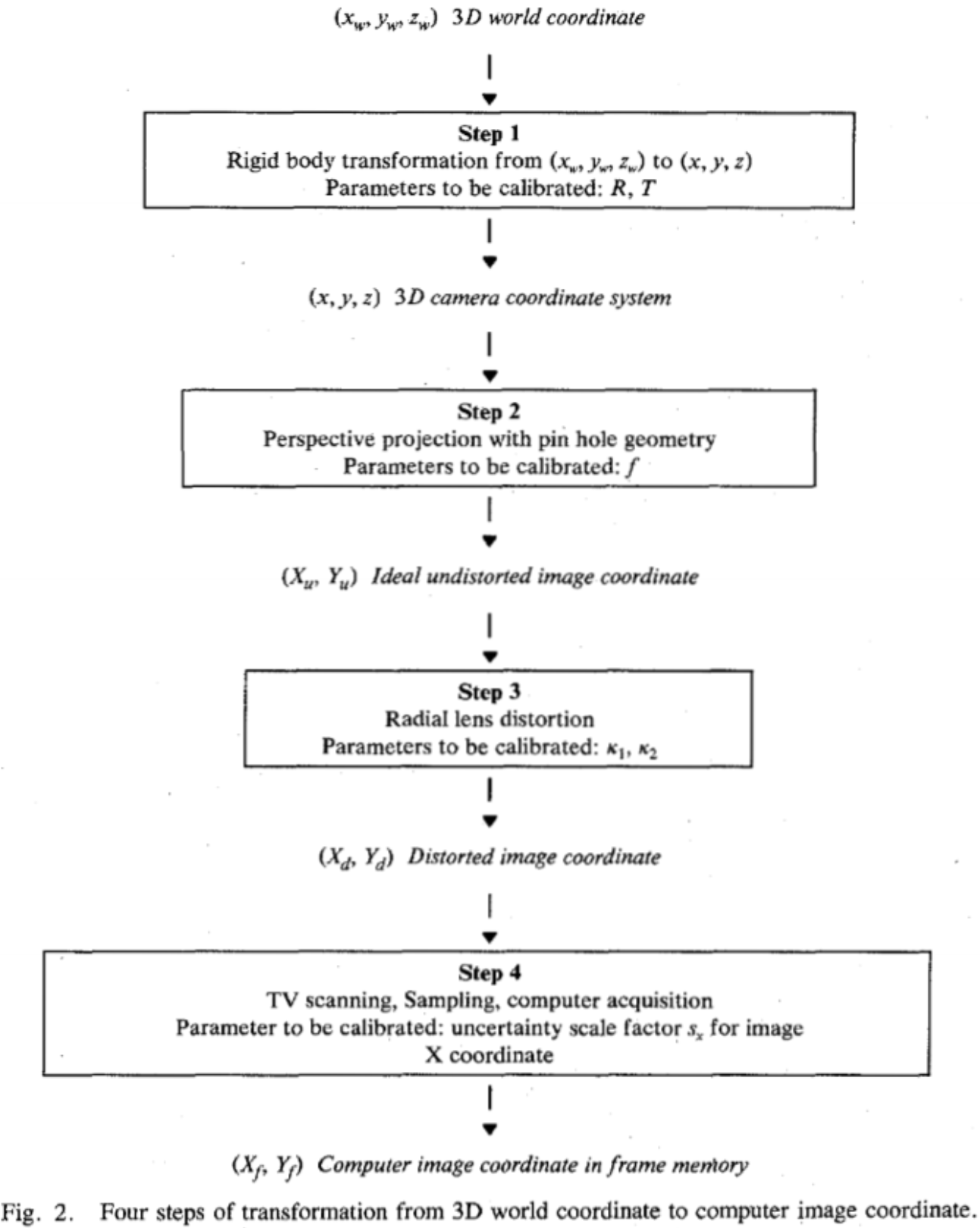
Rigid body transformation from the object world coordinate system $(x_w, y_w, z_w)$ to the camera 3D coordinate system $(x, y, z) $. 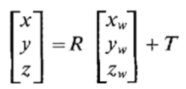. $R,T$ need to be calibrated. Translation is calibrated before rotation.

However, how can one know $(x_w, y_w, z_w)$?
Transformation from 3D camera coordinate$(x, y, z)$ to ideal (undistorted) image coordinate $(X_u, Y_u)$. $X_u=f\frac{x}{z},Y_u=f\frac{y}{z}$.
Calibrate radial lens distortion $k_1,k_2$. Experimentally only one $k$ of radial lens distortion will work fine. The more will cause numerical instability.

$X_d(1+k_1r^2+k_2r^4+\cdots)=X_u,\\Y_d(1+k_1r^2+k_2r^4+\cdots)=Y_u,\\r=\sqrt{X_d^2+Y_d^2}$.
Real image coordinate $(X_d,Y_d)$ to computer image coordinate $(X_f,Y_f)$. $S_x$ is gonna be calibrated.

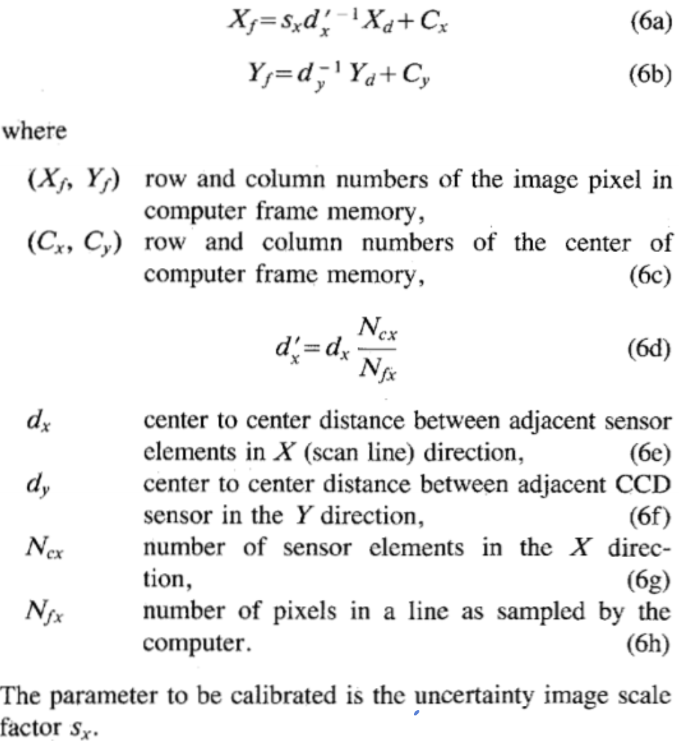
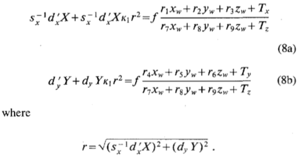
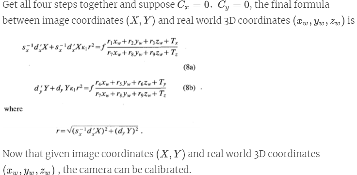
Get all four steps together and suppose $C_x=0，C_y=0$, the final formula between image coordinates $(X,Y)$ and real world 3D coordinates $(x_w,y_w,z_w)$ is

Now that given image coordinates $(X,Y)$ and real world 3D coordinates $(x_w,y_w,z_w)$ , the camera can be calibrated.

Implementation by a monoview coplanar set of points

Before started, make sure $(x_w,y_w,z_w)$ is out of the field view and not close to the $y$ axis so as to avoid $T_y=0$.

Compute 3D Orientation , Position ($x$ and $y$) and sclerosis factor
- Compute the distorted image coordinates $(X_d,Y_d)$
  
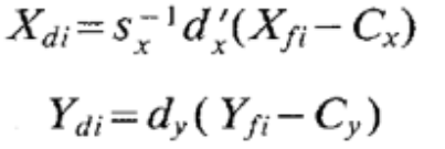  , where $C_x,C_y$ are supposed as the center of the image frame (aka they cannot be calibrated), $s_x$ is not calibrated here but from a priori.
- Compute the five unknowns $T_y^{-1}r_1,T_y^{-1}r_2,T_y^{-1}T_x,T_y^{-1}r_4,T_y^{-1}r_5$.
  
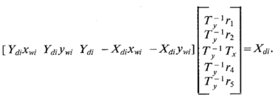  , this requires at least 6 points.
- Compute $(r_1,\cdots,r_9,T_x,T_y)$ from $(T_y^{-1}r_1,T_y^{-1}r_2,T_y^{-1}T_x,T_y^{-1}r_4,T_y^{-1}r_5)$
  - Compute $|T_y|$ from $(T_y^{-1}r_1,T_y^{-1}r_2,T_y^{-1}T_x,T_y^{-1}r_4,T_y^{-1}r_5)$
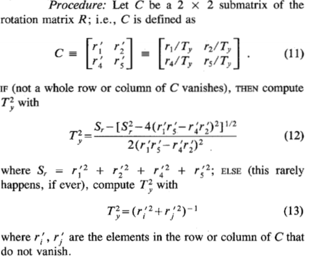
  - Determine the sign of $T_y$.
    
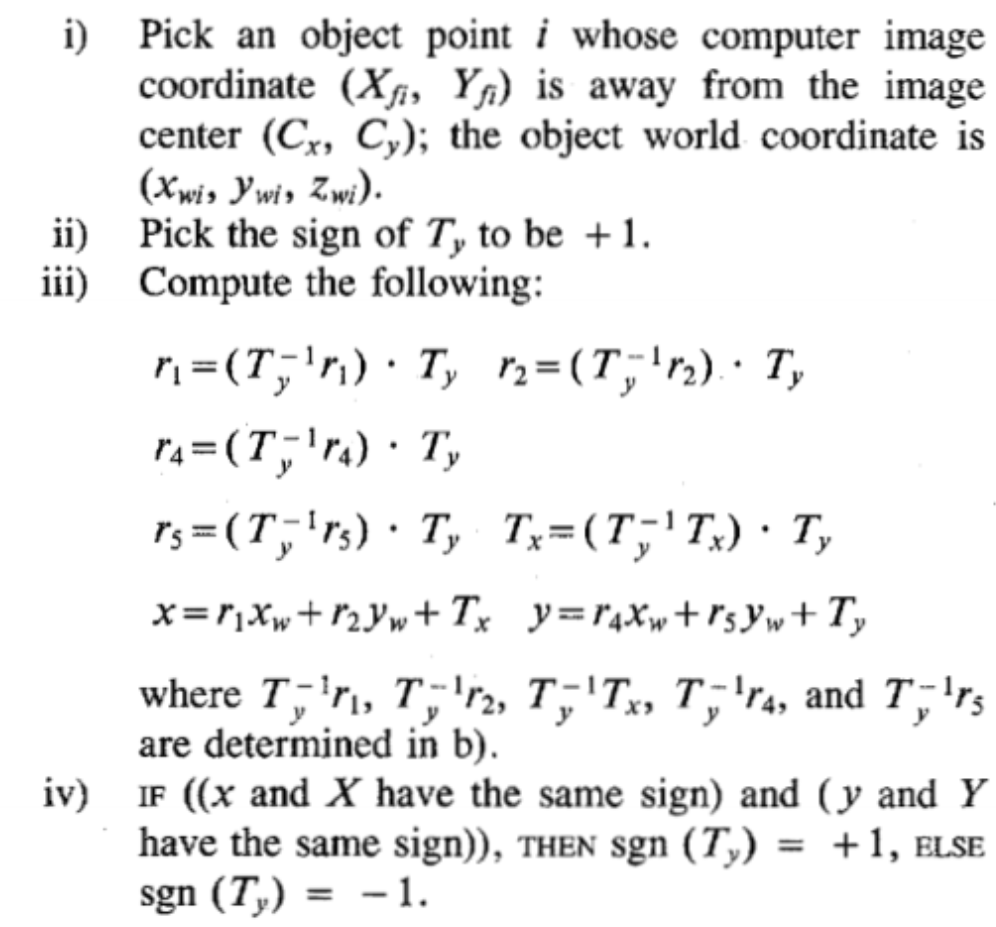
    This sign reversal of $T_y$ causes $(x,y)$ to become $-(x,y)$. But because $X_d,x$ have the same sign, $Y_d, y$ have the same sign, then only one of the two signs for $T_y$ is valid .
  - Compute the 3D rotation $R$
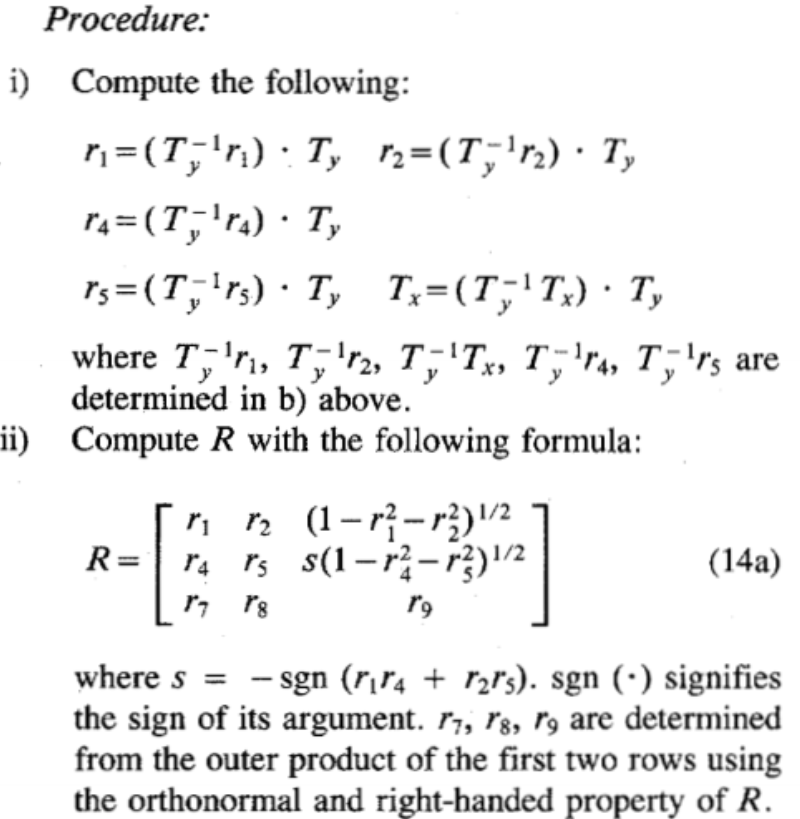
Compute effective focal length, distortion coefficients and $z$ position.

Here, $k_1=0$.
- Compute an approximation of $f, T_z$ by ignoring lens distortion.
- Compute exact solution for $f,T_z,k_1$
  
  Solve $(8b)$: , with $f,T_z,k_1$ as unknowns using standard optimization scheme such as steepest descent. The approximation of $f,T_z$ in previous step can be used as initial guess, and the initial guess of $k_1$ can be taken as zero.

Implementation using monoview noncoplanar points

When $s_x$ is unknown . Now a coplanar set of calibration points is required. Now $z_w$ is no longer identical zero.

Compute 3D Orientation , Position ($x$ and $y$) and scale factor
- Compute the distorted image coordinates $(X_d,Y_d)$ \[ X_{di}={d_x}'(X_{fi}-C_x)\\ Y_{di}=d_y(Y_{fi}-C_y) \] where $C_x,C_y$ are supposed as the center of the image frame (aka they cannot be calibrated), here, the real $s_x$ is absorbed into the unknowns for the liner equation in equations below.
- Compute the seven unknowns $T_y^{-1}s_xr_1,T_y^{-1}s_xr_2,T_y^{-1}s_xr_3,T_y^{-1}s_xT_x,T_y^{-1}s_xr_4,T_y^{-1}s_xr_5,T_y^{-1}s_xr_6$.
  
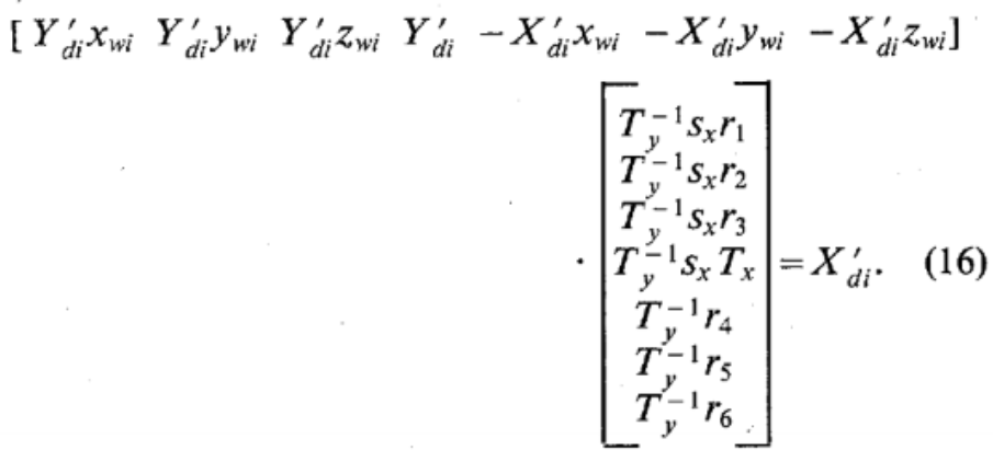  , this requires at least 8 points.
- Compute $(r_1,\cdots,r_9,T_x,T_y)$ from $T_y^{-1}s_xr_1,T_y^{-1}s_xr_2,T_y^{-1}s_xr_3,T_y^{-1}s_xT_x,T_y^{-1}s_xr_4,T_y^{-1}s_xr_5,T_y^{-1}s_xr_6$
  - Compute $|T_y|$ from $(T_y^{-1}r_1,T_y^{-1}r_2,T_y^{-1}T_x,T_y^{-1}r_4,T_y^{-1}r_5)$
  - Determine the sign of $T_y$.
    
    This sign reversal of $T_y$ causes $(x,y)$ to become $-(x,y)$. But because $X_d,x$ have the same sign, $Y_d, y$ have the same sign, then only one of the two signs for $T_y$ is valid .
  - Determine s_x:
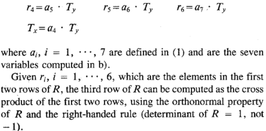
  - Compute the 3D rotation $R$
    
    ,
Compute effective focal length, distortion coefficients and $z$ position.

Here, $k_1=0$.
- Compute an approximation of $f, T_z$ by ignoring lens distortion.
- Compute exact solution for $f,T_z,k_1$
  
  Solve $(8b)$: , with $f,T_z,k_1$ as unknowns using standard optimization scheme such as steepest descent. The approximation of $f,T_z$ in previous step can be used as initial guess, and the initial guess of $k_1$ can be taken as zero.

Paper

3D photography on your desk, 1998, website

Why?

Knowing the 3D shape helps a lot, and the progress and computers and computer graphics also encourage the recovering of 3D shape
Previous
- commercial 3D scanners: accurate but expensive and bulky. Use motorized transport of temporal object and active (laser, LCD projector) lighting of the scene
- Passive cues contain information on 3D shape: stereoscopic disparity, texture, motion parallax, defocus, shadows, shading and specularities, occluding contours and other surface discontinuities amongst them. Stereoscopic disparity is popular way but it suffers from the requirement of two cameras and failing on untextured faces

Goals

Simple and inexpensive approach for extracting the 3D shape of objects

How?

Idea

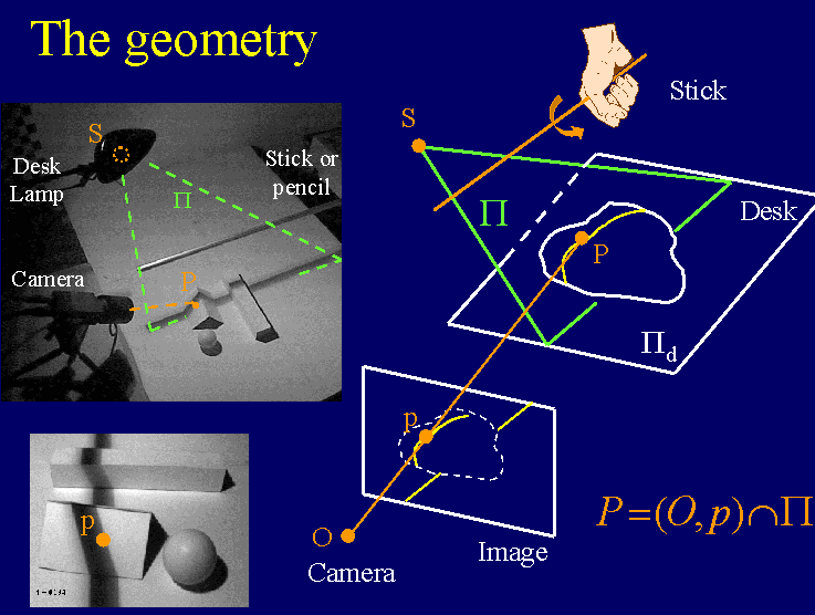
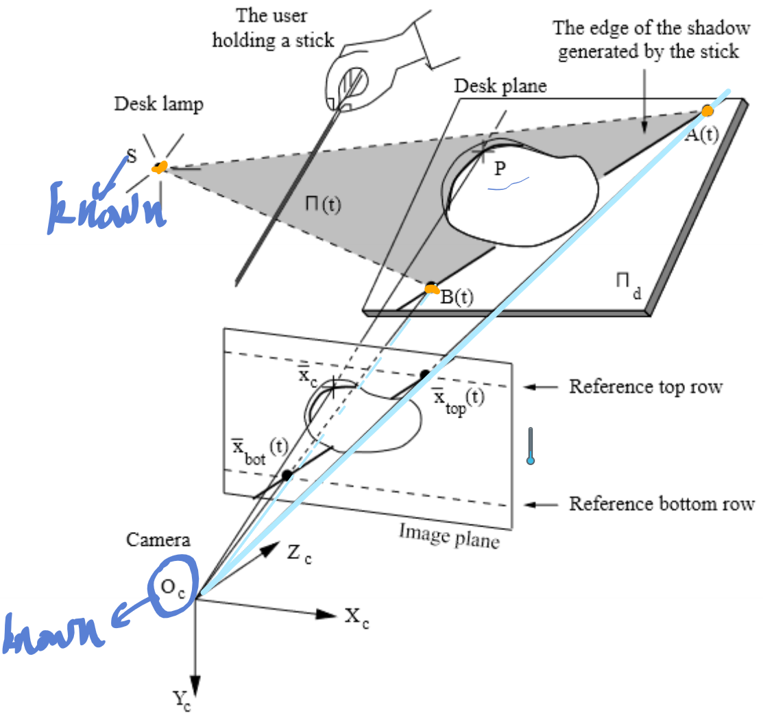
Illuminate the camera (facing the object) by desk-lamp, then the user moves a pencil in front of the light source casting a moving shadow on the object, the 3D shape of object will be recovered by the spatial and temporal location of the observed shadow.

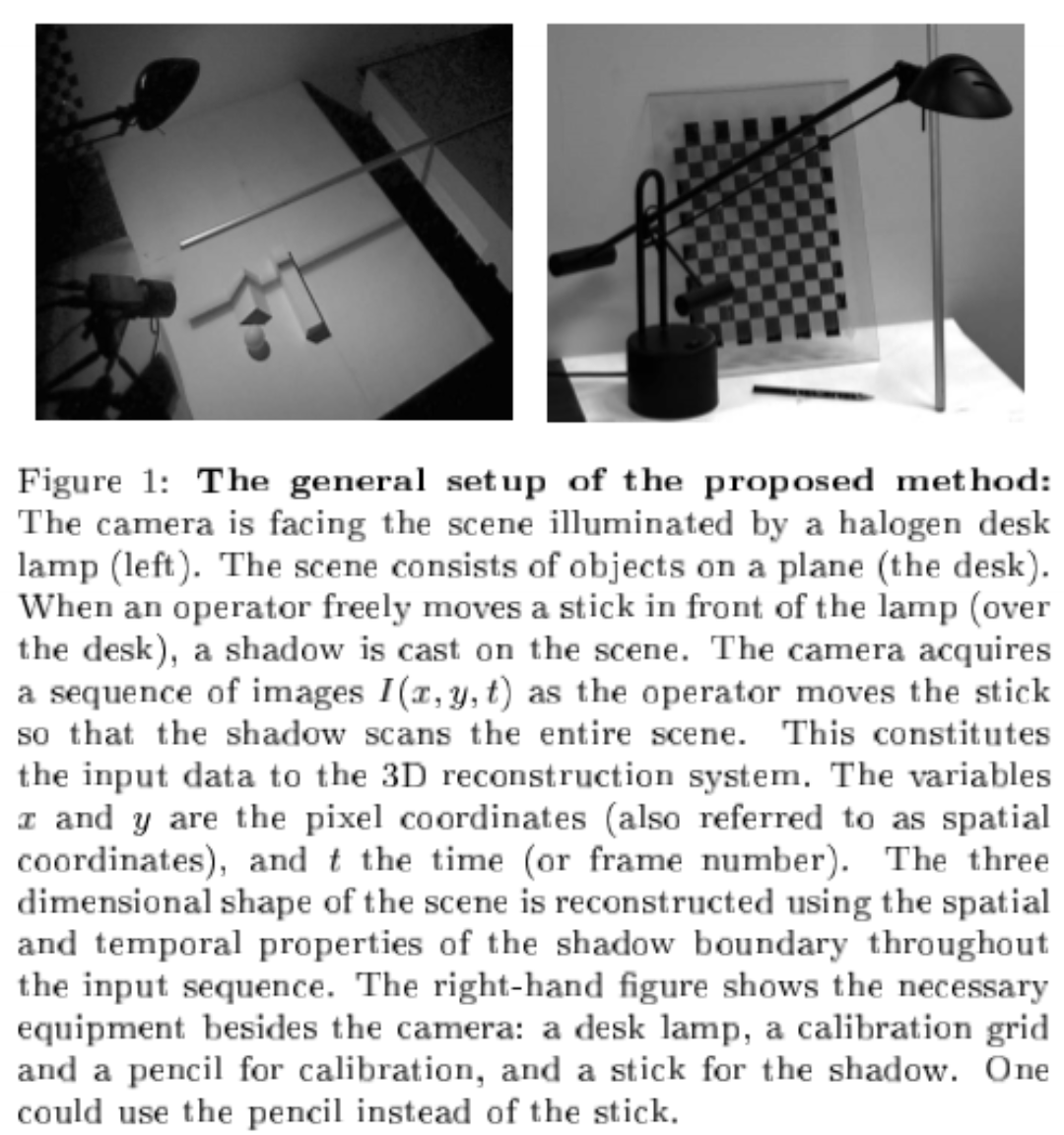
Implementation

Calibration

Camera calibration
- recover the intrinsic camera parameters ($f,K,s_x,(u_0,v_0)$) and the location of the desk plane with respect to camera.
- The method is from here. But because the object used is planar, the optical center cannot be calibrated exactly, so the optical center is assumed to be the center of the image.
  - Specifically, this method considering lens distortion. And the steps for calibration is
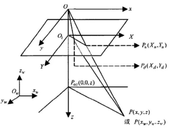
    - Why there are lens distortion ? On some cheap camera, the captured pixel on image is rectangle but not square. This will lead to lens distortion. Under lens distortion, suppose the image point under ideal case is $(X_u,Y_u)$, and after lens distortion the image point is $(X_d,Y_d)$, $K$ is the lens distortion coefficient, then
      
      $r^2={X_u}^2+{Y_u}^2,\\ X_d=X_u(1+Kr^2),Y_d=Y_u(1+Kr^2)$
    - From the image above, $P_u$ is the image coordinates of $P$ in real 3D world under ideal case (no lens distortion ), and $P_d$ is the image coordinates considering lens coordinates. Then the formulas are:
lamp calibration : to determine the 3D location of the point light source $S$
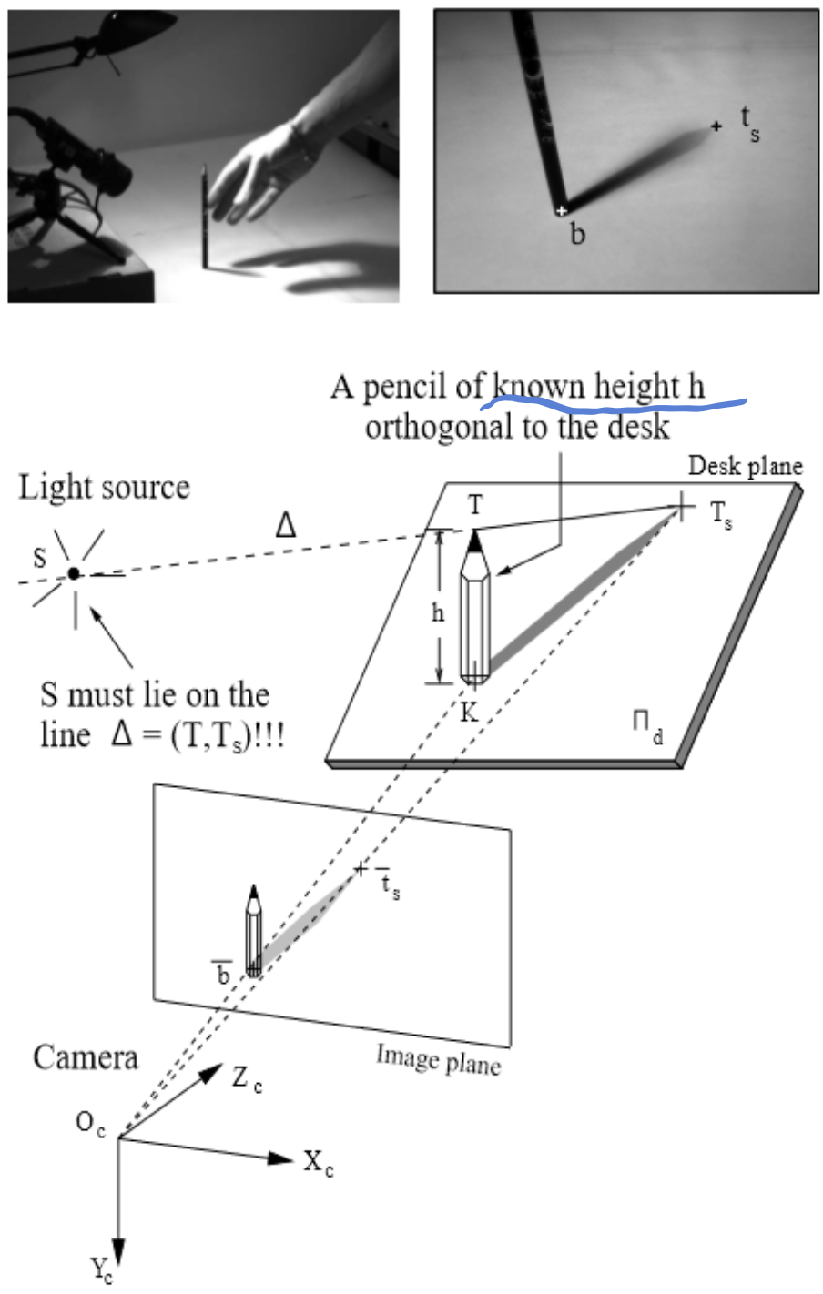
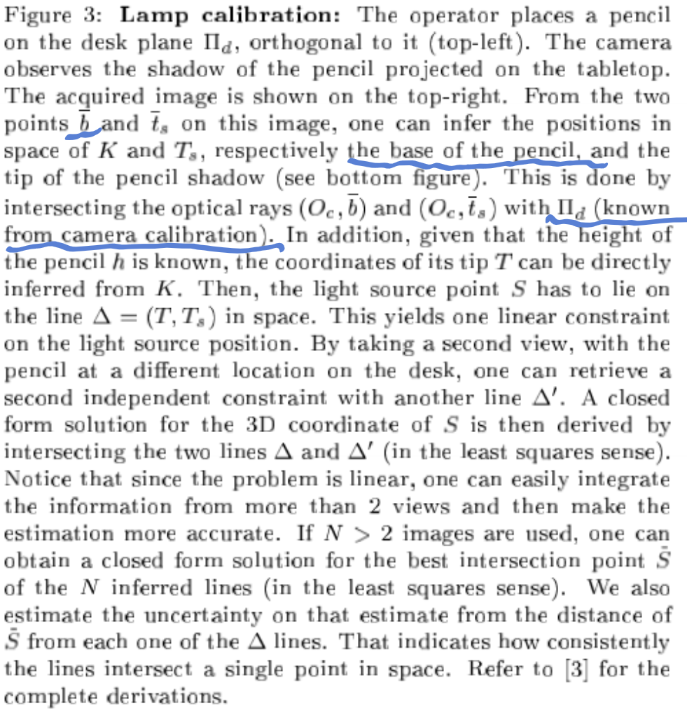
- Given the height of pencil: $h$, the pencil will be orthogonal to the desk.
- Measure the bottom of the pencil ($\bar{b}$) and the tip of the shadow $\bar{t}_s$ in captured image, then according to the calibrated camera, the coordinates of pencil bottom in 3D world (denoted as $K$) and the tip of shadow in real 3D world ($T_s$) can be estimated. Then the tip of pencil in 3D world ($T$) is estimated by $h$.
- The light source $S$ will be the intersection of two rays $TT_S$. Therefore, two position of pencils will help figure the light source out.

Spatial and temporal shadow edge localization

Notice temporal shadow will be scanned from the left to the right side of the scene and thus the right edge of the shadow corresponds to the front edge of the temporal profile

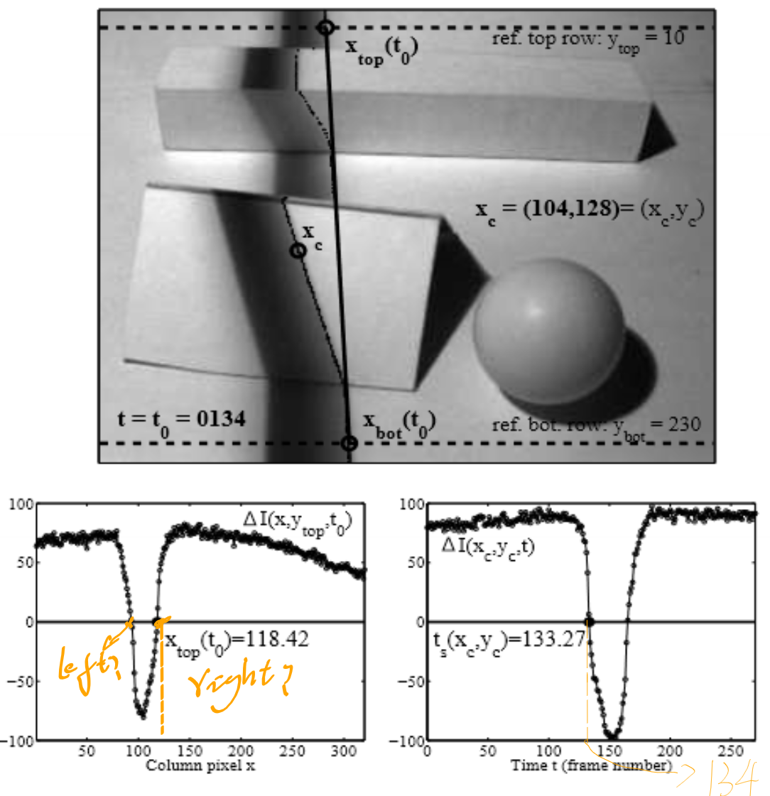
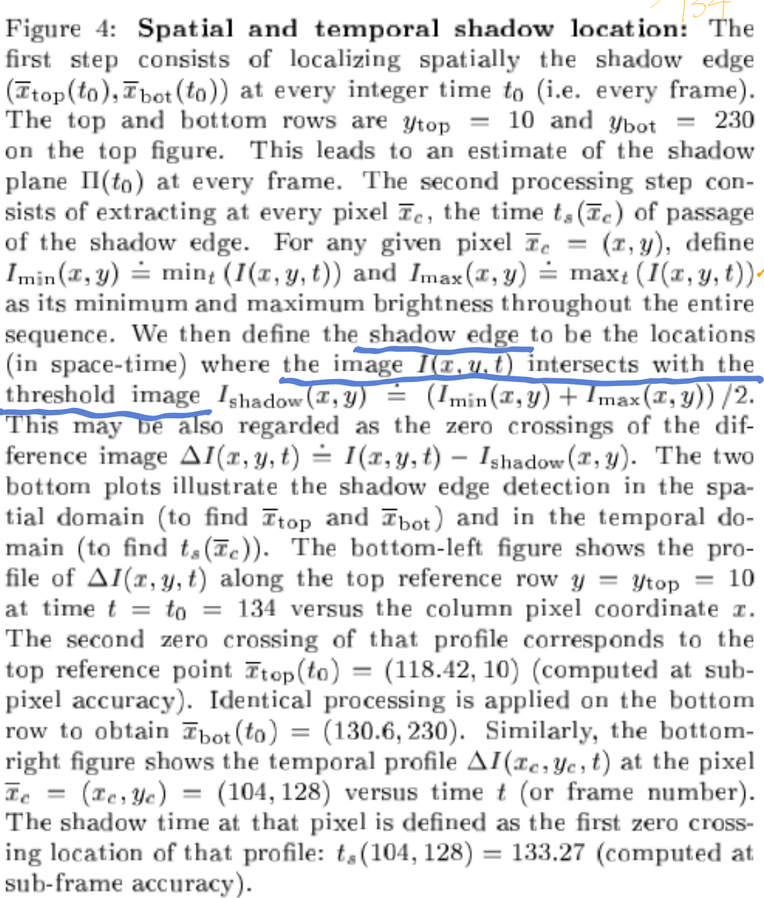
Two steps to be done
- Localize the edge of the shadow that is directly projected on the tabletop $(\bar{x}_{top}(t),\bar{x}_{bot}(t))$ at every time instant $t$ (every frame).
- Estimate the time $t_s(\bar{x}_c)$ (shadow time) where the edge of the shadow passes through any given pixel $\bar{x}_c=(x_c,y_c)$ in the image.
Cause the pixels corresponding to regions in the scene are not illuminated by the lamp, so they don't provide any relevant depth information. And that's why only processing pixels with contrast value ($I_{max}(x,y)-I_{min}(x,y)$) larger than predefined threshold $I_{thresh}$, which is 70 in this paper.
Adaptive threshold image $I_{shadow}(x,y)=(I_{max}(x,y)+I_{min}(x,y))/2$
No spatial filtering is used cause it would generate undesired blending in the final depth estimates.
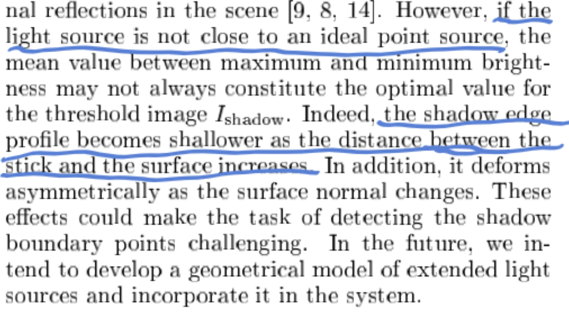
But when the light source is not close to an ideal point source, the predefine threshold $I_{shadow}$ (as a mean) is not optimum. The shadow edge profile becomes shallower as the distance between the stick and the surface increase.
To do it real-time, as the images $I(x,y,t)$ are acquired , one needs to update at each frame five different arrays $I_{max}(x,y),I_{min}(x,y),I_{contrast}(x,y),I_{shadow}(x,y),t_{s}(x,y)$.
- For one pixel $(x,y)$, the maximum brightness $I_{max}(x,y)$ is collected at the 1st frame
- The $I_{min}(x,y), I_{contrast}(x,y)$ is updated as time going. Once $I_{contrast}(x,y)$ crosses $I_{thresh}$ (larger than 70?? which means now there is a shadow on pixel (x,y)?? ), the adaptive threshold $I_{shadow}(x,y)$ starts being computed and updated at every frame. This process goes on till the pixel brightness $I(x,y,t)$ is larger than than $I_{shadow}(x,y)$ at the 1st time. This time instant is registered as the shadow time $t_s(x,y)$.

Triangulation

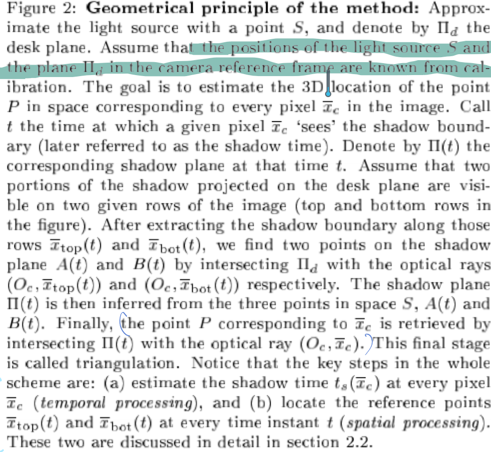
The real 3D point $P$ is gonna be the intersection of line $O_c\bar{x}_c$ and the given pixel $\bar{x}_c$'s shadow plane.
The shadow time $t_s(\bar{x}_c)$ acts as an index to the shadow plane list $\prod(t)$. Besides, the final plane $\prod(t_s(\bar{x}_c))$ will from plane $\prod(t_0-1)$ and $\prod{t_0}$ if $t_0-1<t_s{(\bar{x}_c)}<t_0$ and $t_0$ integer.
After the range data are recovered, a mesh can be used to build the 3D surface.

Noise sensitivity

For quantifying the effect of the noise in the measurement data $\{x_{top}(t), x_{bot}(t), t_{s}(\bar{x}_c)\}$ on the final reconstructed scene depth map, he analysis of the variance of the induced noise on the depth estimation $Z_c$, aka $\sigma_{Z_c}$, will help. In a word, $\sigma_{Z_c}$ can quantify the uncertainties on the depth estimation $Z_c$ at every pixel $\bar{x}_c$, and also constitute a good indicator of the overall accuracies in reconstruction (since most of the errors are located along the $Z$ direction of the camera frame ).
The variance of the induced noise on the depth estimation $Z_c$, aka $\sigma_{Z_c}$, is derived by taking the 1st order derivatives of $Z_c$ with respect to the 'new' noisy input $x_{top},x_{bot},\bar{x}_c$

,
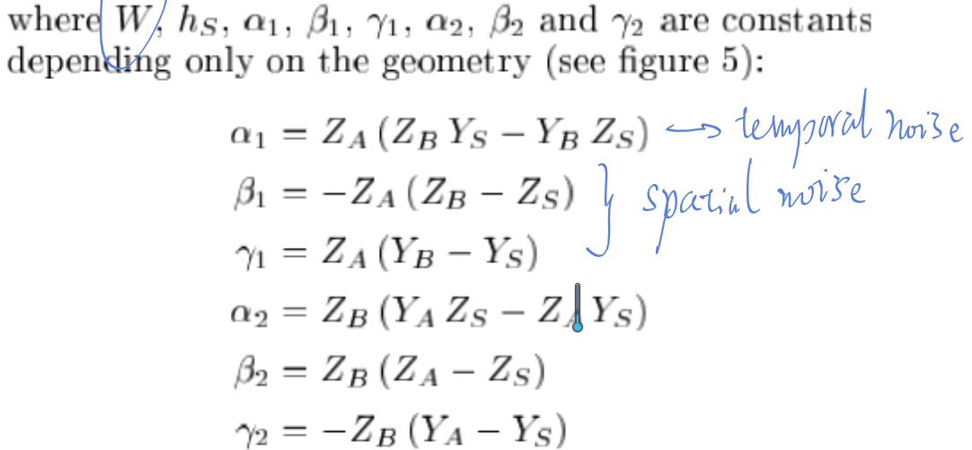
From the equation $\sigma_{x_c}=\frac{\sigma_I}{|I_x(\bar{x}_c)|}$, $\sigma_{x_c}$ does not depend on the local shadow speed. Therefore , decreasing the scanning speed would not increase the accuracy . However, better slow down while scanning when the shadow edge is sharper so as to get good samples for every pixel. But with slow scanning speed, an appropriate low-pass filter before extraction of $t_{s}(\bar{x}_c)$ is required for good accuracy.
Numerically, most of the variations in the variance $\sigma_{Z_c}^2$ are due to the variation of volume $V$ within a single scan. And Therefore the reconstruction noise is systematically larger in portions of the scene further away from the lamp.
- To avoid the systematic error, one may take two scans of the same scene with the lamp at two different locations (on the left and right side of the camera say)
- The final depth is estimated as \[ Z_c=w_LZ_c^L+w_RZ_c^R \] where $Z_c^L,Z_c^R$ are the two estimates (from left and right) of the same depth $Z_c$.
  - If they are gaussian distributed, and independent, then using
  \[ w_L=\frac{\sigma_{Z_R}^2}{\sigma_{Z_R}^2+\sigma_{Z_L}^2}=\frac{\alpha^2}{1+\alpha^2},\\ w_R=\frac{\sigma_{Z_L}^2}{\sigma_{Z_R}^2+\sigma_{Z_L}^2}=\frac{1}{1+\alpha^2},\\ \alpha=\frac{V_L}{V_R} \]
  
  for averaging.
  
  But this suffers from degradation of the overall final reconstruction cause may the $Z_c^L,Z_c^R$ are not gaussian .
  - To avoid the problem mentioned above, another solution is sigmoid. \[ w_L=\frac{1}{1+\exp(-\beta\Delta V)},\\ w_R=\frac{1}{1+\exp(\beta\Delta V)},\\ \Delta V=\frac{V_L^2-V_R^2}{V_L^2+V_R^2}=\frac{\alpha^2-1}{\alpha^2+1} \] The positive coefficient $\beta$ controls the amount of diffusion between the left and the right regions. As $\beta$ tends to infinity, merging reduces to hard decision: $Z_c=Z_c^L$ if $V_L>V_R$ and $Z_c=Z_c^R$ otherwise. This will help reduce tends estimation error and obtain more coverage of the scene.
- The global accuracy depends on the scanning . This paper scan vertically, so the average relative depth error $|\frac{\sigma_{Z_c}}{Z_c}|$ is inversely proportional proportion to $|\cos\xi|$. The best value will be got while $\xi=0, \xi=\pi$. aka lamp standing either tot he right ($\xi=0$ ) or to the left ($\xi=\pi$ ) of the camera.

Issues

Point light source

real-time implementation

while estimating the shadow time

All that one needs to do is update at each frame five different arrays $I_{max}(x; y), I_{min}(x; y), I_{contrast}(x; y),$ $I_{shadow}(x; y)$ and the shadow time $t_s(x; y)$, as the images $I(x; y; t)$ are acquired. For a given pixel $(x; y)$, the maximum brightness $I_{max}(x; y)$ is collected at the very beginning of the sequence (the first frame), and then, as time goes, the incoming images are used to update the minimum brightness $I_{min}(x; y)$ and the contrast $I_{contrast}(x; y)$. Once $I_{contrast}(x; y)$ crosses $I_{thresh}$, the adaptive threshold $I_{shadow}(x; y)$ starts being computed and updated at every frame (and activated). This process goes on until the pixel brightness $I(x; y; t)$ crosses $I_{shadow}(x; y)$ for the first time (in the upwards direction). That time instant is registered as the shadow time $t_s(x; y)$. In that form of implementation, the left edge of the shadow is tracked instead of the right one, however the principle remains the same.

shadow time

Function: works as an index to the shadow plane list so as to using the intersection to locate $P$.
Accuracy: Since $t_s(\bar{x}_c)$ is estimated at sub-frame accuracy, the final plane $\prod(t_s(\bar{x}_c))$ actually results from linear interpolation between the two planes $\prod(t_0-1)$ and $\prod(t_0)$ if $t_0-1 < t_s(\bar{x}_c) < t_0$ and $t_0$ integer.

Accuracy of depth estimation

The accuracy increases as the sharpness of image increases.
Remove the lamp reflector improve the accuracy.
Decreasing the scanning speed would not increase accuracy.
To guarantee the accuracy of sharp edges of object, temporal pixel profile must be sufficiently sampled within the transition area of the shadow edge. Therefore, the sharper the shadow edge, the slower the scanning speed will help.
$\sigma_{Z_c}$ is a good indicator of the overall accuracies while reconstruction, since most of the errors are located along the $Z$ direction of the camera frame.
As the shadow moves into the opposite direction of the lamp, the absolute value of the volume $|V|$ strictly decreases and making $\sigma_{Z_c}$ larger. Therefore, the reconstruction noise is systematically larger in portions of the scene further away from the lamp.

Experiments

Calibration accuracies

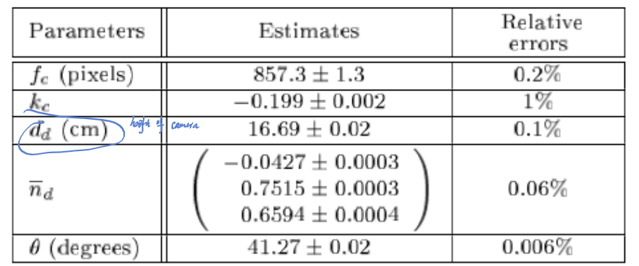
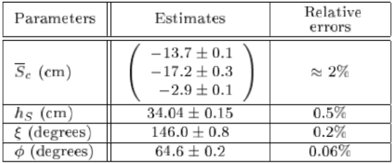
For camera calibration,
- 10 images of the checkboard are taken, nearly 90 corners on the checkboard (8*9).
- the relative error of radial distortion is larger than others.
In lamp calibration,
- collect 10 images of the pencil shadow
- $\bar{S}_c$ is the coordinate vector of the light source in the camera frame, points $b,t_s$ were manually extracted from the images.
- The calibration accuracy is about 3mm, which is sufficient for final shape recovery.

Scene reconstructions

Planarity of the plane
- There is a decrease of approximately $6\%$ in residual standard deviation after quadratic warping. The global geometric deformations are negligible compared to local surface noise. It indicates that the errors of calibration for not induce significant global deformations on the final reconstruction.
- Why 0.23mm/5cm?
Geometry of the corner
- The overall reconstructed structure does not have any major noticeable global deformation.
- The errors (which errors? The surface noise?) are the order of 0.3mm in most experiments.
Angle scene
- With bulb naked, there is a significant improvement in the sharpness of the projected shadow compared the shadow captured with lamp reflector.

Outdoor

outdoors where the sun may be used as a calibrated light source (given latitude, longitude, and time of day).

Conclusion

Simple and low cost system to extracting surface shape of objects. It can be used in real time. The accuracies on the final reconstruction are reasonable (at most $1\%$ or 0.5mm noise error)
it easily scales to larger scenarios indoors and outdoors.
Future work:
- like using the sun as the light source if measuring outdoors.
- multiple view integration so as to move freely the object in front ode the camera and lamp between scans.
- Incorporate a geometrical model of extended light source to the shadow edge detection process.

QA

Briefly explain, referring to the figure, how to obtain a 3D reconstruction at from a camera, a light source, a stick, and one or two shots.
- preliminaries: calibrated lamp $S$ and camera $O_c$.
- Slowly scan the target object by the stick and saved as a video.
  - Do the statistics to get $I_{max},I_{min}$ and then define $I_{shadow}$.
  - Check the video, for the image of each object's point (manually defined, such as each pixel of this object) $\bar{x}_c:(x_{c},y_{c})$ in the whole video, use $I_{shadow}$ and image intensity, draw the temporal shadow and locate the $t_s(x_c,y_c)$ (the index of frame).
- For each point in object $\bar{x}_c$:
  - Check the shadow time $t_s(x_c,y_c)$ and pick the corresponding image.
  - Set $x_{bot}(t), x_{top}(t)$ on the picked image, and then find its corresponding 3D points $A(t),B(t)$ respectively.
  - Define the shadow plane as the plane consists of $S,A(t),B(t)$.
  - The 3D point of $x_c$, denoted as $P$ is the intersection of shadow plane and ray $O_cx_c$.
- After the 3D coordinates of all interested points $\bar{x}_c$ are detected, 3D reconstruction can be completed.
Referring to the figure, explain what the reference points A (t) and B (t) are for.

Points $A(t)$ and $B(t)$ are the 3D points, and used to define the shadow plane by light source $S$ and these two points.
To find the internal and external parameters of the camera, the article offers a method of calibration with a single image of a checkerboard placed on the desktop, but in this case it is necessary know the main point (center of the image). What could we do if we don't know the point and we want to estimate it?
- ~~Method 1：2D-3D calibration~~
  
  Use the dodecahedron as the 3D object to calibrate camera. The optical center is the unknown parameter of camera intrinsic matrix $\mathrm{K}$. Because the DoF of $\mathrm{K}$ is 8, at least 4 pairs of non-coplanar points (2D-3D) are required during calibration.
- Method 2：plane calibration
  
  Still, use the checkboard, but this time move the checkboard so as to get at least two images of checkboard with different pose (keep at least one pose on the desk), each image and checkboard pair will generate at least 4 pairs of 2D-3D points. With at least 2 homographies (induced from the images), the IAC, denoted as $\omega$ can be detected and thus $\mathrm{K}$ is detected by Cholesky decomposition cause $\omega=\mathrm{K}^{-T}\mathrm{K}^{-1}$. The optical center is in $\mathrm{K}$.
The article says that if we use two planes perpendicular ($\pi_h$ and $\pi_v$) rather than a single plane, we do not need calibrate the light source. Why?

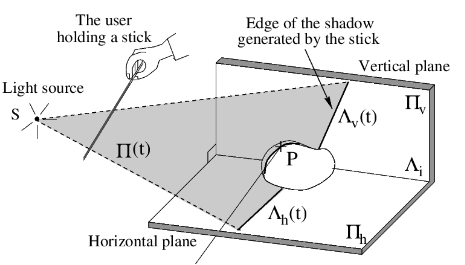
The requirement of light source $S$ is for the detection of shadow plane so as to get the intersection of shadow plane and ray $O_cx_c$. Three non-coplanar points define a plane. Here, $A(t), B(t)$ are detected by calibrated camera $O_c$ and images of them. Suppose $A(t),B(t)$ is on $\pi_v$ and any one shadow point $S'$ is on $\pi_h$. Since $\pi_h \perp\pi_v$, $S'$ is easy to be detected. Armed with these three points $A(t),B(t), S$, the shadow plane can be located.
Why must the light source used be “point”? Explain. Give an example of a non-point light source that would also be adequate.
- If the light source is not close to an ideal point source, the mean value between maximum and minimum brightness may not always constitute the optimal value for the threshold image $I_{shadow}$. Indeed, the shadow edge profile becomes shallower as the distance between the stick and the surface increases. In addition, it deforms asymmetrically as the surface normal changes. These effects could make the task of detecting the shadow boundary points challenging.
- naked bulb: like just remove the lamp reflector in paper.
The article says that if we use a vertical pencil, we can calibrate the light source. Explain how, based on the illustration to the right. State how many images are needed and explain why.
- Given the height of pencil: $h$, the pencil will be orthogonal to the desk.
- Measure the bottom of the pencil ($\bar{b}$) and the tip of the shadow $\bar{t}_s$ in captured image, then according to the calibrated camera, the coordinates of pencil bottom in 3D world (denoted as $K$) and the tip of shadow in real 3D world ($T_s$) can be estimated. Then the tip of pencil in 3D world ($T$) is estimated by $h$.
- The light source $S$ will be the intersection of two rays $TT_S$. Therefore, two position of pencils will help figure the light source out.
Explain the concepts of temporal shadow and spatial shadow and what are their roles in the reconstruction process.
- spatial shadow helps to detect the column index of $A(t),B(t)$'s images. After finding this, the real position of $A(t),B(t)$ can be detected by the calibrated camera $O_c$ and the shadow plane can be defined also. Then the 3D coordinates can be detected as the intersection of shadow plane and ray $O_cx_c$.
- temporal shadow works as an index to the shadow plane list so as to using the intersection to locate $P$.
Explain for the following elements of the assembly how it could be modified and to improve the precision of the 3D reconstruction. In each case, justify your answers.
- choice of light source:
  - point light source, like what mentioned in the paper just remove the lamp reflector. Or can use candle without reflector. May can also use a board with only one small hole in front of the light, but this should be adjusted to make sure all required shadows are created (difficult in practical). The reason is a point light source creates more precise shadows.
  - may can move the light source further away from the object to make shadow more clear.
- choice of stick used to shade:
  
  make sure the edge of stick is sharp (like a square stick), and long enough to cover the target object. Because the sharper the stick, its shadow edge will be more clear and easier to be detected and thus to locate $\bar{x}_{bot},\bar{x}_{top}$. The long enough stick will generate required shadow.
- spatial resolution of the camera (image size):
  
  the higher the spatial resolution, the more detailed the image (more pixels and smaller points), and thus the more detailed the reconstruction. To make sure the high spatial resolution, one can decrease the distance between camera and object or fix the camera but prolong the focal length.
- temporal resolution of the camera (number of images per second):
  
  make the scan speed faster will increase the temporal resolution. The sharper the shadow edge, the higher the temporal resolution will help. If the scan speed is too fast, then one can see a blurred shadow that hurts the reconstruction accuracy, but this can be fixed by reducing the exposure.
The article suggests that the same method can be used outdoors. Based on the illustration to the right, explain how this can be done.
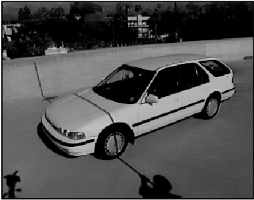
- Calibration of light source (sun) and camera
  - The camera calibration can be done by checkboard.
  - The calibration of light source: use the latitude, longitude, and cause the sun is very far away from the earth, each ray can be taken as a parallel ray.
- Take the video of shadow image and take the note of time of the day. Similarly, calculate $I_{max},I_{min}$ and then calculate $I_{shadow}$. Draw the temporal profile and denote the shadow time $t_s(x_c,y_c)$ as the time of day.
- For each point in object $\bar{x}_c$:
  - Check the shadow time $t_s(x_c,y_c)$ and pick the corresponding image.
  - Set $x_{bot}(t), x_{top}(t)$ on the picked image, and then find its corresponding 3D points $A(t),B(t)$ respectively.
  - Define the shadow plane as the plane consists of $S,A(t),B(t)$.
  - The 3D point of $x_c$, denoted as $P$ is the intersection of shadow plane and ray $O_cx_c$.
- After the 3D coordinates of all interested points $\bar{x}_c$ are detected, 3D reconstruction can be completed.