泛函
不动点定理
不动点定理的基本逻辑:对于一个存在性问题,构造一个度量空间和一个映射,使得存在性问题等价于这个映射的不动点。只要证明这个映射存在不动点,那么原来的存在性问题即得证。
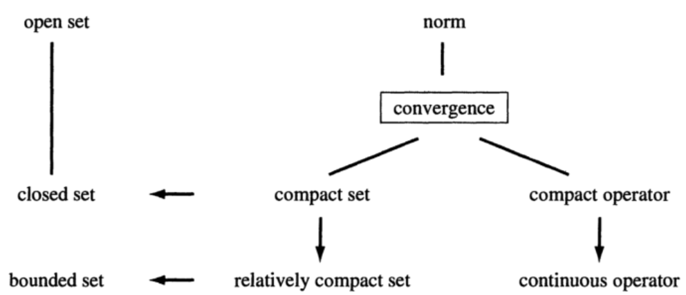
紧性的利用
- 证明存在性
- 在无限维空间中“模仿”有限维的欧式空间
紧集是为了模仿描述欧式空间中的有界闭集合么? 紧=相对紧+闭
流形(Manifolds)
- 概念:高维空间中曲线、曲面概念的推广,如三维空间中的曲面为一二维流形。
支撑集(Support)
- 概念:函数的非零部分子集;一个概率分布的支撑集为所有概率密度非零部分的集合
数学分析
Lipschitz连续
- 若存在一个常数K,使得定义域内的任意两点x1,x2满足: $ |f(x_1)-f(x_2)|=K|x_1-x_2|$ 则称函数为Lipschitz连续函数。此性质限定了f的导函数的绝对值不超过K,规定了函数的最大局部变动幅度。
Statistical learning theory
Introduction
Determine how well a model performs on unseen data
Preliminary
Markov Inequality
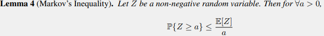 , in the order of \(\mathcal{O}(\frac{1}{deviation})\)
Chebyshev's Inequality
 , in the order of \(\mathcal{O}(\frac{1}{deviation^2})\)
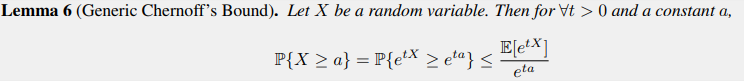
Generic Chernoff's Bound
Hoeffding's Inequality
Hoeffding's lemma

Hoeffding's Inequality
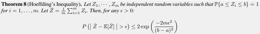
Hoeffding's inequality is useful to bound the probability of the gap between an empirical value and the true expectation of an average of bounded random variables.
McDiarmid's Inequality
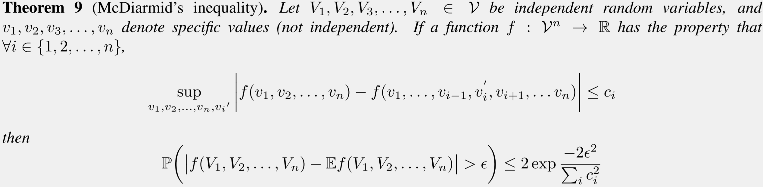
- A concentration inequality.
- This bound is useful because if we prove that an algorithm is β stable then we will have this property on a specific function.
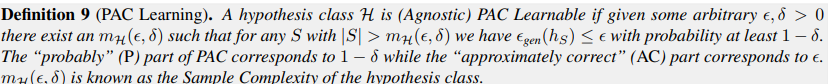
PAC
Check here for PAC, VC, uniform bound and others.
PAC Learning (agnostic PAC learnable)--finite hypothesis class
- Consider a simple linear classifier with 2 weights \(\vec{w} = (w_1;w_2)\), which are stored using a 32 bit floats. This implies that the hypothesis class is finite with $|| = 2^{32} $.
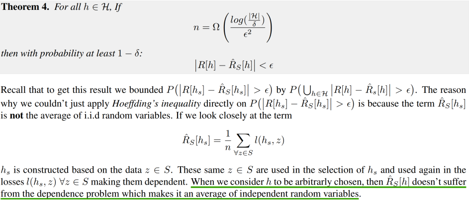
- This theorem works on finite hypothesis class, and answers that for a hypothesis class \(\mathcal{H}\), to make the generation gap is smaller than \(\epsilon\) with at least \(1-\delta\), the required samples complexity.
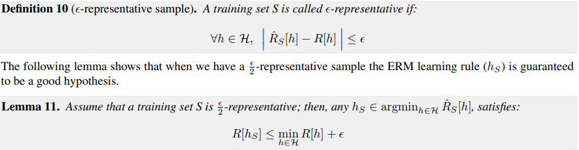
- Once a hypothesis class is PAC learnable, with high probability the training set is \(\epsilon\)-representative.
- Note Suppose \(\mathcal{H}\) is PAC learnable, there is not a unique function \(m_{\mathcal{H}}\) that satisfies the requirements given in the definition of PAC learnability.
- Finite classes are PAC Learnable, also agnostic PAC Learnable.
Uniform convergence
- Formalize that over all hypothesis in \(\mathcal{H}\), the empirical risk is close to the true risk. This will make sure the ERM to work.
VC dimension
measure the complexity of hypothesis class other than cardinality.
Shattering

VC Dimension

Informally VC dimension is the maximum number of distinct points that a hypothesis in \(\mathcal{H}\) can correctly classify every possible labeling with zero error.
- With infinite VC dimension, the hypothesis class won't be PAC learnable.
- There exist hypothesis classes with uncountable cardinality but finite VC dimension.
- For every two hypothesis classes if \(\mathcal{H}_0 \subset \mathcal{H}\) then \(VCdim(\mathcal{H}_0) \leq VCdim(\mathcal{H})\).
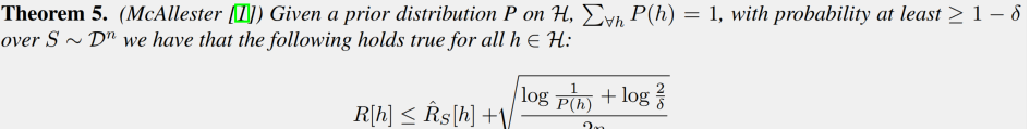
Occam's bound
The PAC bound can be treated as Occam's bound with a uniform prior .
Occam's bound will put a distribution over the countably infinite hypothesis class \(\mathcal{H}\) that is independent of dataset \(S\) we will receive. In doing so we will get bounds on the generalization gap that no longer depend on the size of the hypothesis class, \(|\mathcal{H}|\). These bounds now become variable depending on how we weigh each individual hypothesis \(h\), i.e. \(P(h)\).
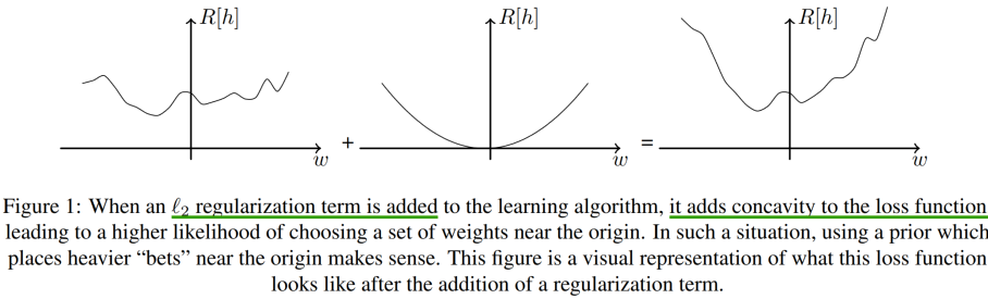
Regularizers offers higher probability assigned to \(\vec{w}\) near the origin and thus a tighter bound, it won't influence the algorithm (loss). Specifically , when an \(\ell_2\) regularization term is added to the learning algorithm, it adds concavity to the loss function.
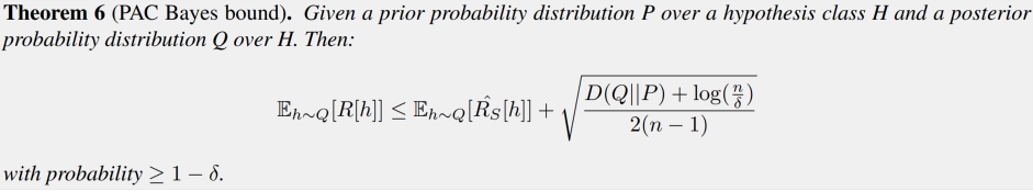 , where \(D(Q\|P)\) is the KL divergence which serves as a complexity measure.
It tells that with a good posterior that is close to the prior, then the KL-divergence will become smaller and out bound will be tighter. Even though it's tight, the bound is tight for hypothesis that we may not care about, e.g. tight on the bound with respect to \(P\) prior on hypothesis.
Note that the posterior is after applying the prior \(P\) on hypothesis, and seeing the data, then one can get this posterior \(Q\).
Why posterior?
different choices of prior and posterior hypotheses can be made, each resulting in a new bound without us touching the algorithm.
The dropout PAC-Bayes is a lower bound on the PAC-Bayes bound that becomes tight when the dropout factor is 0.
Stability, Generalization
PAC learning and Occam's bound work as algorithm-agnostic bounds.
Stability
Hint: a change in data distribution does not change the predictions.
Definition: uniform stability

An algorithm with this property can be understood as one that produces a hypothesis such that the loss function \(\ell\) is not drastically affected by perturbing the dataset in this manner.
EMR with regularization is \(\beta\)-stable.
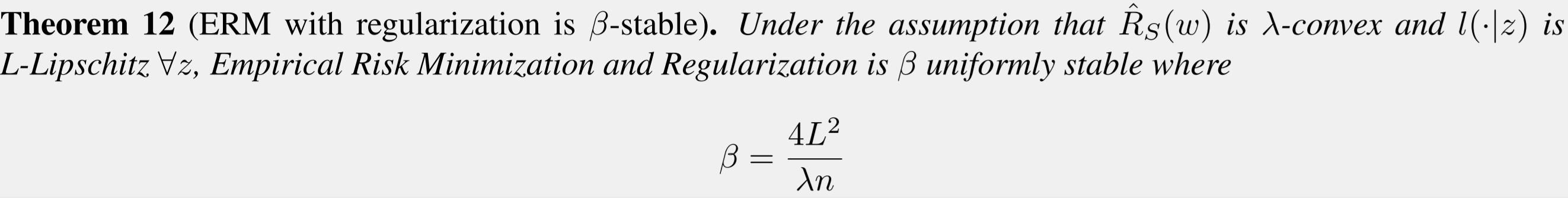
- If we perturb the data by a single element, we learn \(\mathcal{A}\) that can become arbitrarily close for large \(n\).
SGD is stable
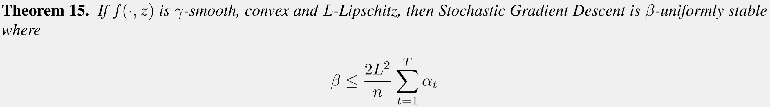
- It holds for a finite number of steps \(T\)
Defect:
\(D[h_S]=R[h_S]-\hat{R}_S[h_S]\)
Defect \(D[h_S]\) for a hypothesis \(h_S\) derived from an algorithm after seeing the dataset \(S\) is defined as the difference between the population risk and the empirical risk.
It's expectation is not zero.
The expectation value of defect can be bounded under certain conditions.
If $ $ is a \(\beta\)-uniformly stable algorithm, then \(-\beta\le \mathbb{E}[D[h_S]]\le\beta\).
Let \(\mathcal{A}\) be a \(\beta\)-uniformly stable learning algorithm with respect to a loss function \(\ell:\mathcal{Y\times Y}\rightarrow [0,M]\). The absolute difference of the defect calculated on a dataset \(S\) and on a perturbed version of the dataset \(S^{i,z}\) is bounded by \(|D[h_S]-D[h_{S^{i,z}}]|\le 2\beta +\frac{M}{n}\).
For a \(\beta\)-uniformly stable algorithm, the relationship between the empirical and the population risk is \(\mathbb{E}[R[h_S]]\le\mathbb{E}_S[\hat{R}_S[h_S]]+\beta\).
- It's a bound on the expectation value of the population risk. But this bound does not hold for all possible \(h_S\).
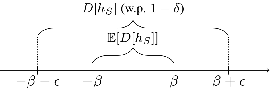
For a \(\beta\)-uniformly stable algorithm \(\mathcal{A}\) with respect to a loss function \(\ell:\mathcal{Y\times Y}\rightarrow [0,M]\) and a hypothesis \(h_S\) with \(|S|=n\). The relationship between the empirical and the population risk holds with probability \(1-\delta\): \(R[h_S]\le \hat{R}_S[h_S]+\beta +(n\beta+\frac{M}{2})\sqrt{\frac{2\log\frac{2}{\delta}}{n}}\).
- The last term is a concentration Inequality (McDiramid's)
- For this bound, as \(n\) goes up, it becomes less tight.
Convex Optimization
Book Convex Optimization, Convex Optimization: Algorithms and Complexity
| Terminology | Definition |
|---|---|
| Convex function: origin | \(f(\theta x+(1-\theta)y)\le \theta f(x)+(1-\theta)f(y)\) |
| Convex function: 1st order (once differential ) | $f(y)f(x)+f(x)^T (y-x) $ |
| Convex function: 2nd order (twice differential ) | \(\nabla^2f(x)\succeq0\), the eigenvalues won't be negative |
| \(L\)-Lipschitz | \(\|f(x)-f(y)\|\le L\|x-y\|\) |
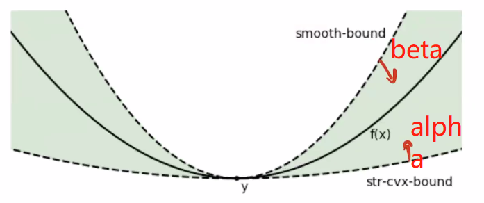
| \(\beta\)-smooth: \(\beta\)-Lipschitz on gradient | \(\|\nabla f(x)-\nabla f(y)\|\le \beta\|x-y\|\Rightarrow \nabla^2f(x)\preceq\beta\mathrm{I}\) |
| \(\alpha\)-strong convex, limited the domain mostly. | \(f(y)-f(x)\le\nabla f(x)^T (y-x)-\frac{\alpha}{2}\|y-x\|^2\Rightarrow \nabla^2f(x)\succeq\alpha\mathrm{I}\) |
| Optimizer | Condition | Converge rate | Optimal step size | Sub-optimal gap | Bounds of the gap |
|---|---|---|---|---|---|
| GD after \(T\) steps | L-Lipschitz convex | \(\mathcal{O}(\frac{1}{\sqrt{T}})\) | \(\gamma=\frac{\|x_1-x^*\|_2}{L\sqrt{T}}\) | \(f(\frac{1}{T}\sum\limits_{k=1}^{T}x_k)-f(x^*)\) | \(\le\frac{\|x_1-x^*\|L}{\sqrt{T}}\), the initial point matters |
| GD | \(\beta\)-smooth +convex |
\(\mathcal{O}(\frac{1}{T})\) | \(\gamma=\frac{1}{\beta}\), constant and independent of \(T\) |
\(f(x_k)-f(x^*)\) Notice the average on all samples can be erased |
\(\le\frac{2\beta\|x_1-x^*\|^2}{k-1}\), \(k\) means the \(k\) step. Bound depends on initial point |
| Projected subGD after \(T\) steps | \(\alpha\)-strong + \(L\)-Lipschitz |
\(\mathcal{O}(\frac{1}{T})\) | \(\gamma_k=\frac{2}{\alpha (k+1)}\), diminish at every step |
\(f(\sum\limits_{k=1}^T\frac{2k}{T(T+1)}x_k)-f(x^*)\) | \(\le\frac{2L^2}{\alpha (T+1)}\) |
| GD | \(\lambda\)-strong + \(\beta\)-smooth |
\(\mathcal{O}(\exp{(-T)})\) | \(\gamma=\frac{2}{\lambda+\beta}\) | \(f(x_{t+1})-f(x^*)\) Notice the average on all samples can be erased |
\(\le\frac{\beta}{2}\exp{(-\frac{4t}{\kappa+1})}\|x_1-x^*\|^2\), $ =\(. <br />\)k$ is the same meaning of \(t\), rather than the \(\kappa\) in denominator. |
| Polyak (heavy ball) | Quadratic loss | \(\mathcal{O} ((\frac{\sqrt\kappa-1}{\sqrt\kappa+1})^t)\\\approx\exp(-\frac{C}{\sqrt\kappa})\), \(\kappa=\frac{h_{max}}{h_{min}}\) |
\(\gamma^*=\frac{(1+\sqrt\mu)^2}{h_{max}}\\=\frac{(1-\sqrt\mu)^2}{h_{min}}\) | \(\left\|\left[ \begin{matrix} x_{t+1}-x*\\ x_t-x^* \end{matrix} \right]\right\|_2\) | \(\le\mathcal{O} (\rho(A)^T)=\mathcal{O} (\sqrt{\mu}^T)\). \(\mu\) is the curvature |
| Nesterov NAG | \(\beta\)-smooth | \(\mathcal{O}(\frac{1}{T^2})\) | \(f(y_t)-f(x^*)\) | ||
| Nesterov NAG | \(\alpha\)-strong +\(\beta\)-smooth |
\(\mathcal{O}(\exp(-\frac{T}{\sqrt{\kappa}}))\) | \(f(y_t)-f(x^*)\) | \(\le\frac{\alpha+\beta}{2}\|x_k -x^*\|^2\exp(-\frac{t-1}{\sqrt\kappa})\) | |
| SGD | \(L\)-Lipschitz by \(\|\tilde{g}(x)\|\le L\) with prob. 1 |
\(\mathcal{O}(\frac{1}{\sqrt T})\) If wants a \(\epsilon\)-tolerance, \(T\ge\frac{B^2L^2}{\epsilon^2}\) |
\(\gamma=\frac{B}{L\sqrt{T}}\) | \(\mathbb{E}[f(\bar{x})]-f(x^*)\), where \(x^*\in\arg\min_{x:\|x\|<B}f(x)\) |
\(\le\frac{BL}{\sqrt T}\) |
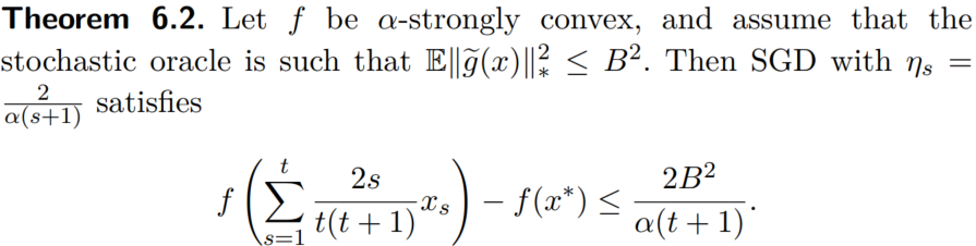
| SGD | \(\alpha\)-strong+ \(\mathbb{E}\|\tilde{g}(x)\|_*^2\le B^2\) (kind of \(B\)-smooth) | \(\mathcal{O}(\frac{1}{T})\) | \(\gamma=\frac{2}{\alpha(s+1)}\) | \(f(\sum\limits_{s=1}^t\frac{2s}{t(t+1)}x_s)-f(x^*)\) | \(\le\frac{2B^2}{\alpha(t+1)}\) |
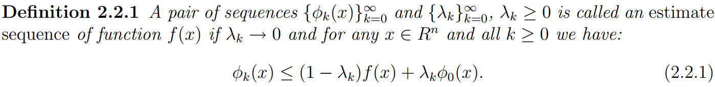
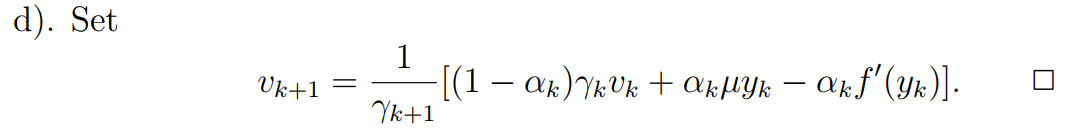
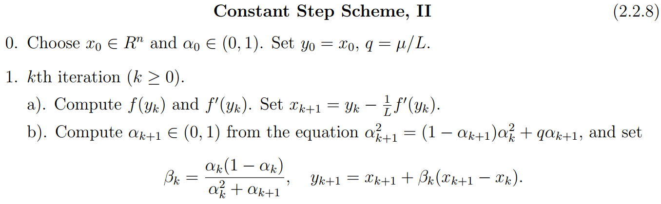
Estimate sequence
Definition
Properties
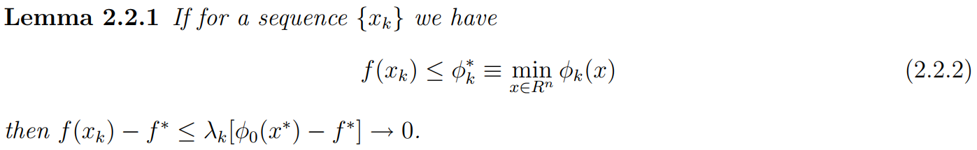
for any sequence \(\{\lambda_k\}\), satisfying \((2.2.2)\) we can derive the rate of convergence of the minimization process directly from the rate of convergence of the sequence \(\{\lambda_k\}\).
Note: below in estimate sequence, all \(L\) means \(L\)-smooth function
How to form an estimate sequence?
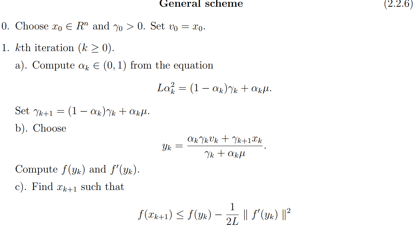
How to ensure \((2.2.2)\)?
Method 1: Do scheme (2.2.6), it will generate a sequence \(\{x_k\}_{k=0}^\infin\) such that \(f(x_k)-f^*\le \lambda_k[f(x_0)-f^*+\frac{\gamma_0}{2}\|x_0-x^*\|^2]\). It will make sequence satisfy \((2.2.2)\)
Method 2: Using gradient step
Some cases
- If in the scheme (2.2.6) we choose \(\gamma_0\ge\mu\), then \(\lambda_k\le\min\{(1-\sqrt{\frac{\mu}{L}})^k,\frac{4L}{(2\sqrt{L}+k\sqrt{\gamma})^2}\}\).
- If in the scheme (2.2.6) we choose \(\gamma_0=L\), then this scheme generates a sequence \(\{x_k\}_{k=0}^{\infin}\) such that \(f(x_k)-f^*\le L\min \{(1-\sqrt{\frac{\mu}{L}})^k,\frac{4}{(k+2)^2}\}\|x_0-x^*\|^2\). This means that it's optimal for the class \(\mathcal{S}_{\mu,L}^{1,1}(R^n)\) with \(\mu\ge0\).
- If in the scheme \((2.2.8)\) we choose \(\alpha_0\ge \sqrt{\frac{\mu}{L}}\), then this scheme generates a sequence \(\{x_k\}_{k=0}^{\infin}\) such that \(f(x_k)-f^*\le \min \{(1-\sqrt{\frac{\mu}{L}})^k,\frac{4L}{(2\sqrt{L}+k\sqrt{\gamma_0})^2}\}[f(x_0)-f^*+\frac{\gamma_0}{2}\|x_0-x^*\|^2]\), where \(\gamma_0=\frac{\alpha_0(\alpha_0L-\mu)}{1-\alpha_0}\). Here \(\alpha_0\ge \sqrt{\frac{\mu}{L}}\) is equivalent to \(\gamma_0\ge\mu\).
Convex sets
Affine sets
- Affine sets:
- Definition : A set \(C\subseteq R^n\) is affine if the line through any two distinct points in \(C\) lies in \(C\), aka for any \(x_1 ,x_2\in C\) and \(\theta\in R\), one has \(\theta x_1+(1-\theta)x_2\in C\). It indicates that the \(C\) contains the linear combination of any two points in \(C\).
- Induction: If \(C\) is an affine set, \(x_1,\cdots,x_k\in C\) and \(\theta_1+\cdots+\theta_k=1\), then the point \(\theta_1 x_1+\cdots+\theta_kx_k\) also belongs to \(C\).
- Affine hull
- Definition: the set of all affine combinations of points in some set \(C\subseteq R^n\), denoted as \(\mathrm{aff}C\)
- It's the smallest affine set that contains \(C\)
- Affine dimension
- Definition: as the dimension of its affine hull.
- E.g.: \(\{x\in R^2|x_1 ^2+x_2^2=1\}\), the affine dimension is 2.
Convex sets
- Definition: If every point in the set can be seen by every other point, along an unobstructed straight path between them, where unobstructed means lying in the set.
- Every affine set is also convex.
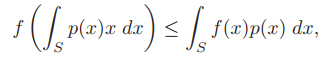
- Convex hull, denotes as \(\mathrm{conv} C\), is the set of all convex combinations of points in \(C\). It is always convex, and it's the smallest convex set that contains \(C\)
- More generally, suppose \(p: R^n \rightarrow R\) satisfies \(p(x)\ge0\) for all \(x\in C\) and \(\int_Cp(x)dx=1\), where \(C\subseteq R^n\) is convex, then \(\int_Cp(x)x dx \in C\), if the integral exists.
Convex functions
Convex functions
Definition
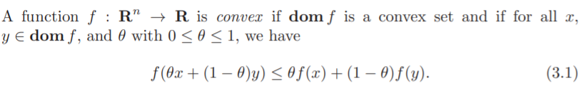
All affine function are both convex and concave.
\(f\) is convex if and only if for all \(x\in \mathrm{dom}f\) and all \(v\), the function \(g(t)=f(x+tv)\) is convex.
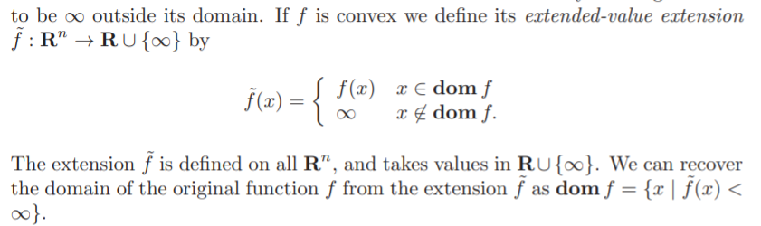
Extended-value extensions
First-order conditions
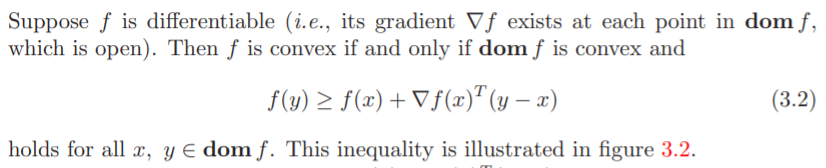
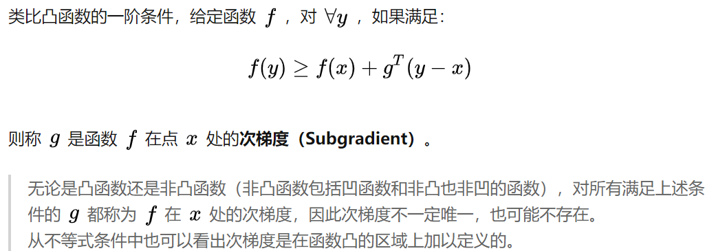
The inequality (3.2) states that for a convex function, the first-order Taylor approximation is in fact a global underestimator of the function. Conversely, if the first-order Taylor approximation of a function is always a global underestimator of the function, then the function is convex.
- The inequality (3.2) shows that if \(\nabla f(x) = 0\), then for all \(y \in \mathrm{dom} f, f(y) ≥ f(x)\), i.e., \(x\) is a global minimizer of the function \(f\).
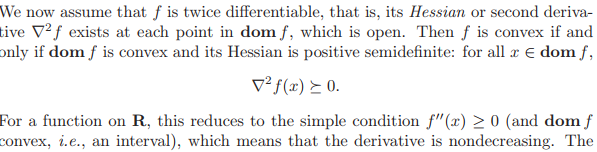
Second-order conditions
More constraints on convex function
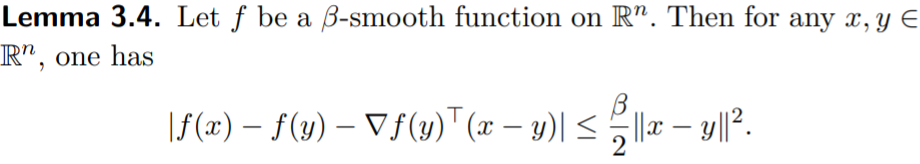
\(\beta\)-smooth
- Definition: a continuously function \(f\) is \(\beta\)-smooth if the gradient \(\nabla f\) is \(\beta\)-Lipschitz, that is \(\|\nabla f(x)-\nabla f(y)\|\le\beta\|x-y\|\).
- If \(f\) is twice differentiable then this is equivalent to the eigenvalues of the Hessians being smaller than \(\beta\) at any point. , \(\nabla^2f(x)\preceq\beta \mathrm{I}_n,\forall x\).
- smoothness removes dependency from the averaging scheme
- If extend the \(\beta\)-smooth to multi power, it's called Holder condition
- The bigger your function changes in gradients, the upper you have to explore.
\(\alpha\)-strong convexity
Strong convexity can significantly speed-up the convergence of first order methods.
Definition
We say that \(f:\mathcal{X}\rightarrow\mathbb{R}\) is a \(\alpha\)-strongly convex if it satisfies the following improved subgradient inequality:
\(f(x)-f(y)\le\nabla f(x)^T(x-y)-\frac{\alpha}{2}\|x-y\|^2\). A large value of \(\alpha\) will lead to a faster rate. A \(\alpha\)-strong convexity for twice differential function \(f\) can also be interpreted as \(\nabla^2f(x)\succeq\alpha \mathrm{I}_n,\forall x\).
Strong convexity plus \(\beta\)-smoothness will lead to the gradient descent with a constant step-size achieves a linear rate of convergence, precisely the oracle complexity will be \(O(\frac{\beta}{\alpha}\log(1/\varepsilon)), \beta\ge\alpha\). In some sense strong convexity is a dual assumption to smoothness, and in fact this can be made precise within the framework of Fenchel duality.
\(\alpha\) can often be reviewed as large as the sample size. Thus reducing the number of step from sample size to \(\sqrt{\mathrm{sample \quad size}}\) (cause \(\kappa=\frac{\beta}{\alpha}\) for \(\beta\)-smooth and \(\alpha\)-strong function, and in basic gradient descent algorithm, to reach \(\epsilon\)-accuracy, it requires \(\mathcal{O}(\kappa\log(\frac{1}{\epsilon}))\), and for Nesterov's Accelerated Gradient Descent attains the improved oracle complexity of \(\mathcal{O}(\sqrt{\kappa}\log(\frac{1}{\epsilon}))\)) can be a huge deal, especially in large scale applications.
Examples of Convex functions
- Norms
- Max function
- Quadratic-over-linear function \(\frac{x^2}{y}\)
- Log-sum-exp: \(\log(e^{x_1}+\cdots+e^{x_n})\), which is regarded as a differentiable approximation of the max function
- Geometric mean: \((\prod\limits_{i=1}^{n}x_i)^{1/n}\), concave
- Log-determinant: \(\log\det X\), concave
For proofs, check Chapter \(3.1.5\) of Convex Optimization.
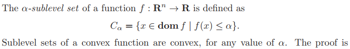
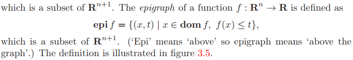
Sublevel sets
Epigraph
A function is convex if and only if its epigraph is a convex set.
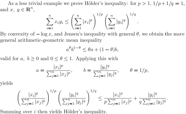
Jensen's inequality and extensions
Once a function is convex, then you can get
 the simplest version of it is \(f(\frac{x+y}{2})\le\frac{f(x)+f(y)}{2}\).
Holder's inequality
Operations that preserve convexity
Nonnegative weighted sums: \(f=w_1f_1+\cdots+w_mf_m\)
Composition with an affine mapping: \(g(x)=f(Ax+b)\). If \(f\) is convex, so is \(g\); if \(f\) is concave, so is \(g\).
Pointwise maximum and suprenum: \(f(x)=\max\{f_1(x),f_2(x)\}\) and \(f(x)=\max\{f_1(x),\cdots,f_m(x)\}\)
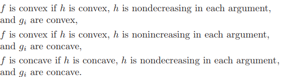
Composition: \(f(x)=h(g(x))\)
Scalar composition
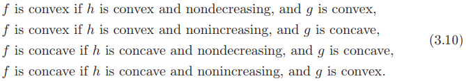
Vector composition \(f(x)=h(g(x))=h(g_1(x),\cdots,g_k(x))\)
Minimization
Typical Numerical optimization
Gradient descent
The basic principle behind gradient descent is to make a small step in the direction that minimizes the local first order Taylor approximation of \(f\) (also known as the steepest descent direction). This kind of methods will obtain an oracle complexity independent of the dimension.
\(x_{t+1}=x_t-\eta\nabla f(x_t)\)
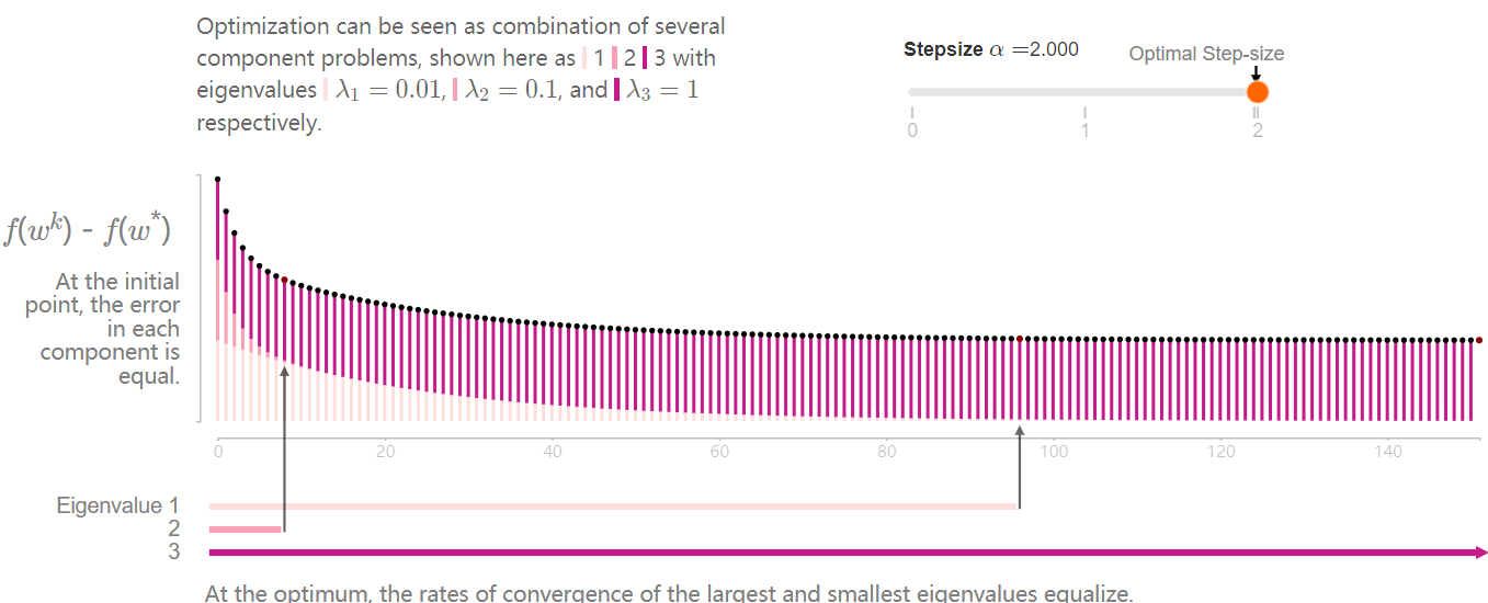
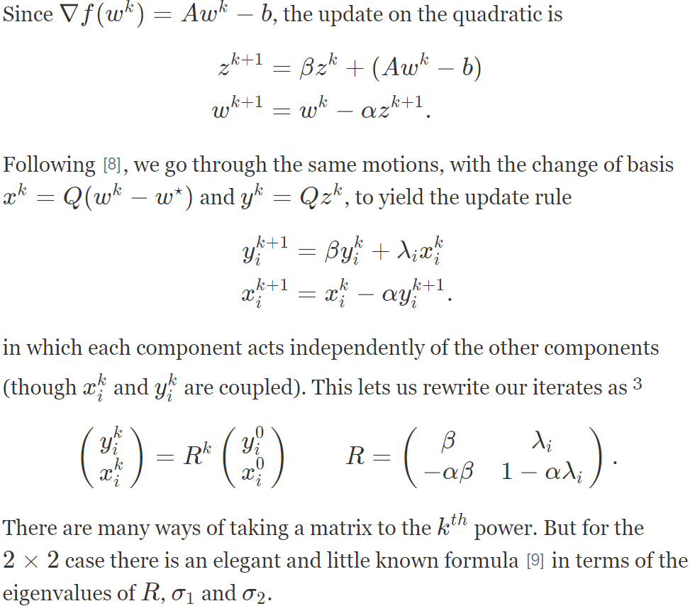
Taking \(f(w)=\frac{1}{2}w^TAw-b^Tw,w\in\mathbb{R}^n\) into consideration, suppose \(A\) is symmetric and invertible, then \(A=Q\Lambda Q^T,\Lambda=(\lambda_1,\cdots,\lambda_n),\lambda_1\le\lambda_2\le\cdots\le\lambda_{n-1}\le\lambda_n\).
All errors are not made equal. Indeed, there are different kinds of errors, \(n\) to be exact, one for each of the eigenvectors of \(A\).
\(f(w^k)-f(w^*)=\sum(1-\alpha\lambda_i)^{2k}\lambda_i[x_i^0]^2\)
Denote the condition number \(\kappa=\frac{\lambda_n}{\lambda_1}\), then the bigger the \(\kappa\) is, the slower gradient descent will be, cause the condition number is a direct description of pathological curvature.
The optimal step-size causes the first and last eigenvectors to converge at the same rate.
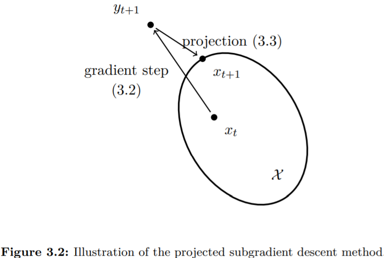
Projected gradient descent
Subgradient
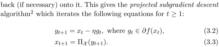
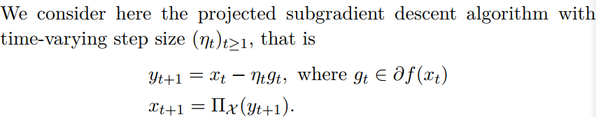
Projected subgradient descent
Gradient descent with momentum : Polyak's Momentum
Sometimes SGD fail with a reason of pathological curvature of objective. (like valley, trench)
Momentum modify gradient descent by adding a short-term memory
\(y_{t+1}=\beta y_t+\nabla f(x_t)\\x_{t+1}=x_{t}-\alpha y_{t+1}\).
When \(\beta=0\), it's gradient descent.
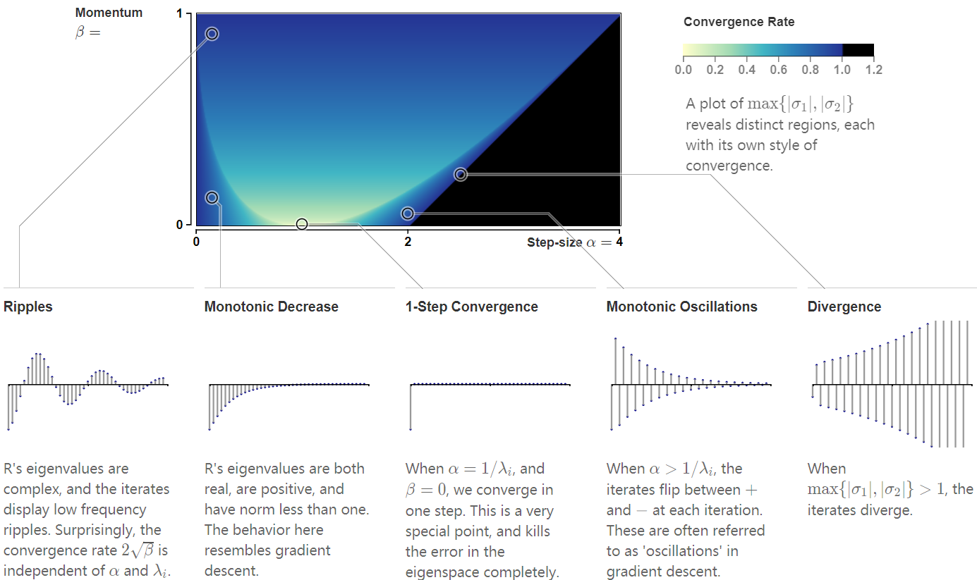
Momentum allows us to crank up the step-size up by a factor of 2 before diverging.
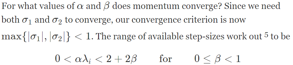
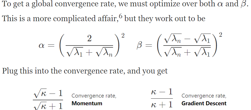
Optimize over \(\beta\): The critical value of \(\beta = (1 - \sqrt{\alpha \lambda_i})^2\) gives us a convergence rate (in eigenspace \(i\)) of \(1 - \sqrt{\alpha\lambda_i}\). A square root improvement over gradient descent, \(1-\alpha\lambda_i\)! Alas, this only applies to the error in the \(i^{th}\) eigenspace, with \(\alpha\) fixed.
Failing: there exist strongly-convex and smooth functions for which, by choosing carefully the hyperparameters \(\alpha\) and \(\beta\) and the initial condition \(x_0\), the heavy-ball method fails to converge.
Nesterov’s Accelerated Gradient Descent
Iterations: starting at an arbitrary initial point \(x_1=y_1\)
\[y_{s+1}=x_s-\frac{1}{\beta}\nabla f(x_s),\\x_{s+1}=(1+\frac{\sqrt{\kappa}-1}{\sqrt{\kappa}+1})y_{s+1}-\frac{\sqrt{\kappa}-1}{\sqrt{\kappa}+1}y_s\]
Let \(f\) be \(\beta\)-smooth and \(\alpha\)-strongly convex, then Nesterov's gradient descent satisfies for \(t\ge0\), \(f(y_t)-f(x^*)\le\frac{\alpha+\beta}{2}\|x_1-x^*\|^2\exp{(-\frac{t-1}{\sqrt{\kappa}})}\) .
Converge in \(\mathcal{O}(\frac{1}{T^2})\) for smooth case, and \(\mathcal{O}(\exp(-\frac{T}{\sqrt{\kappa}}))\), it guaranteed convergence for quadratic functions (and not piece-wise quadractic)
Stochastic gradient descent
Cases: one is \(\mathbb{E}_{\xi}\nabla_x\ell(x,\xi)\in\part f(x)\), where \(\xi\) is sampled. This method cannot be reproduced; the other is directly minimize \(f(x)=\frac{1}{m}\sum\limits_{i=1}^{m}f_i(x)\), here gradient is reported as \(\nabla f_I(x)\), where \(I\in[m]\), this method can be reproduced.
Non-smooth stochastic optimization
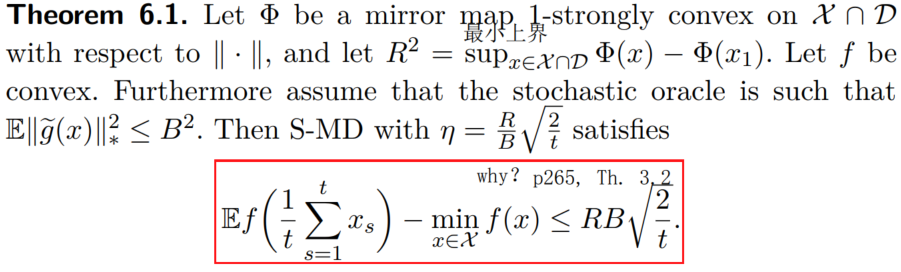
- Definition: there exists \(B>0\) such that \(\mathbb{E}\|\tilde{g}(x)\|_*^2\le B^2\) for all \(x\in\mathcal{X}\)
Smooth stochastic optimization and mini-batch SGD
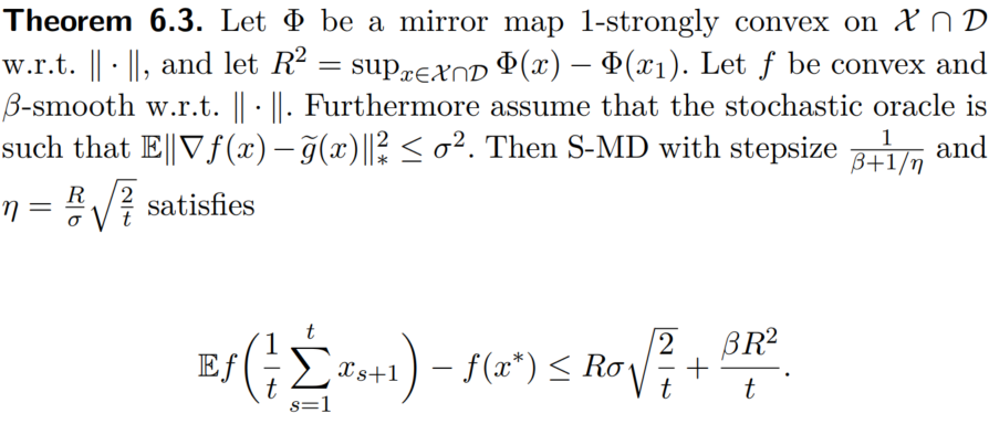
Definition: there exists \(\sigma>0\) such that \(\mathbb{E}\|\tilde{g}(x)-\nabla f(x)\|_*^2\le \sigma^2\) for all \(x\in\mathcal{X}\).
smoothness does not bring any acceleration for a general stochastic oracle , while in exact orale case it does.
Stochastic smooth optimization converge in \(\frac{1}{\sqrt{t}}\). Deterministic smooth optimization converge in \(\frac{1}{t}\)
Mini-batch SGD converges between \(\frac{1}{\sqrt{t}}\) and \(\frac{1}{t}\).
Relations
Generalization
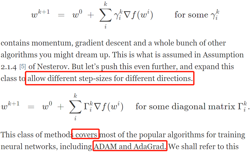
The momentum SGD and Adaptive optimizers
YellowFin and the Art of Momentum Tuning
- Summary: hand-tuning a single learning rate and momentum makes it competitive with Adam. The proposed YellowFin (an automatic fine tuner for momentum and learning rate in SGD), can converge in fewer iterations than Adam on ResNets and LSTMs for image recognition, language modeling and constituency parsing.
- Adaptive optimizers: like Adam, AdaGrad, RmsProp
- For details of paper check here
Dimension-free convex optimization
Projected subgradient descent for Lipschitz functions
Theorem
Assume that \(\mathcal{X}\) is contained in an Euclidean ball centered at \(x_1\in \mathcal{X}\) and of radius \(R\). Assume that \(f\) is such that for any \(x\in \mathcal{X}\) and of any \(g\in\part f(x)\) (assume \(\part f(x)\ne \emptyset\)) one has \(\|g\|\le L\). (This implies that \(f\) is L-Lipschitz on \(\mathcal{X}\), that is \(\|f(x)-f(y)\|\le L\|x-y\|\))
The projected subgradient descent method with \(\eta=\frac{R}{L\sqrt{t}}\) satisfies \(f(\frac{1}{t}\sum\limits_{s=1}^{t}x_s)-f(x^*)\le\frac{RL}{\sqrt{t}}\)
Proof
The rate is unimprovable from a black-box perspective.
Gradient descent for smooth functions
Theorems under unconstrained cases
In this section all \(f\) is a convex and \(\beta\)-smooth function on \(\mathbb{R}^n\).
Theorem
Let \(f\) be convex and \(\beta\)-smooth function on \(\mathbb{R}^n\). Then gradient descent with \(\eta=\frac{1}{\beta}\) satisfies \(f(x_t)-f(x^*)\le\frac{2\beta\|x_1-x^*\|^2}{t-1}\) .
For the proof check \(3.2\) in Convex Optimization: Algorithms and Complexity.
Gradient descent attains a much faster rate in \(\beta\)-smooth situation than in the non-smooth case of the previous section.
The Definition of smooth convex functions
The constrained cases
This time consider the projected gradient descent algorithm \(x_{t+1}=\prod_{\mathcal{X}}(x_t-\eta\nabla f(x_t))\)
- Lemma
Let \(x,y\in \mathcal{X},x^+=\prod_{\mathcal{X}}(x-\frac{1}{\beta}\nabla f(x))\) and \(g_{\mathcal{X}}(x)=\beta (x-x^+)\) , then the following holds true: \(f(x^+)-f(y)\le g_{\mathcal{X}}(x)^T(x-y)-\frac{1}{2\beta}\|g_{\mathcal{X}}(x)\|^2\).
- Theorem
Let \(f\) be convex and \(\beta\)-smooth function on \(\mathcal{X}\). Then projected gradient descent with \(\eta=\frac{1}{\beta}\) satisfies \(f(x_t)-f(x^*)\le\frac{3\beta\|x_1-x^*\|^2+f(x_1)-f(x^*)}{t}\) .
Strong convexity
Strongly convex and Lipschitz functions
- Theorem
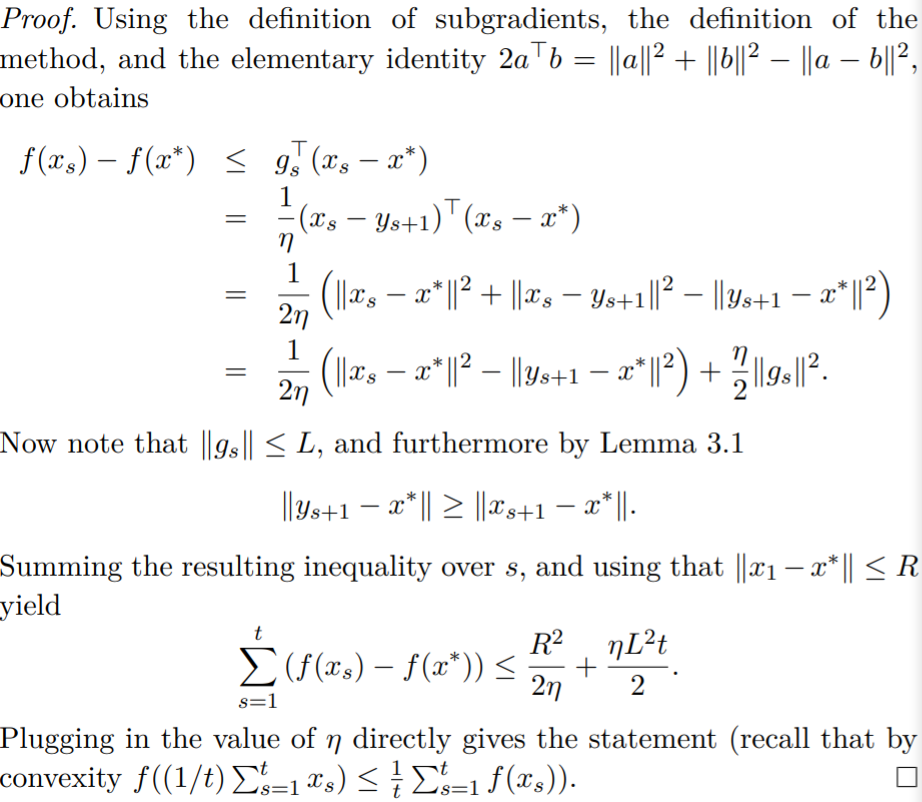
Let \(f\) be \(L\)-Lipschitz and \(\alpha\)-strongly convex on \(\mathcal{X}\). Then projected gradient descent with \(\eta_s=\frac{2}{\alpha(s+1)}\) satisfies \(f(\sum\limits_{s=1}^{t}\frac{2s}{t(t+1)}x_s)-f(x^*)\le\frac{2L^2}{\alpha(t+1)}\) .
The combination of \(\alpha\)-strongly convex and \(L\)-Lipschitz means that function has to be constrained in a bounded domain.
Strongly convex and smooth functions
Theorem
Let \(f\) be \(\beta\)-smooth and \(\alpha\)-strongly convex on \(\mathcal{X}\), then projected gradient descent with \(\eta=\frac{1}{\beta}\) satisfies for \(t\ge0\), \(\|x_{t+1}-x^*\|^2\le\exp(-\frac{t}{\kappa})\|x_a -x^*\|^2\) .
The intuition of changing \(\alpha\) and \(\beta\): If increasing \(\beta\), the upper bound will be decreased, and if increasing \(\alpha\), the lower bound will be increased.
Lemma
Let \(f\) be \(\beta\)-smooth and \(\alpha\)-strongly convex on \(\mathbb{R}^n\), then for all \(x,y\in \mathbb{R}^n\), one has \((\nabla f(x)-\nabla f(y))^T(x-y)\ge\frac{\alpha\beta}{\alpha+\beta}\|x-y\|^2+\frac{1}{\beta+\alpha}\|\nabla f(x)-\nabla f(y)\|^2\) .
Theorem
Let \(f\) be \(\beta\)-smooth and \(\alpha\)-strongly convex on \(\mathbb{R}^n\), \(\kappa=\frac{\beta}{\alpha}\) as the condition number. Then gradient descent with \(\eta=\frac{2}{\beta+\alpha}\) satisfies \(f(x_{t+1})-f(x^*)\le\frac{\beta}{2}\exp(-\frac{4t}{\kappa+1}\|x_1-x^*\|^2)\)
Lower bound -- black box
A black-box procedure is a mapping from "history" to the next query point, that is it maps (\(x_a ,g_1,\cdots,x_t,g_t\)) (with \(g_s\in\part f(x_s)\)) to \(x_{t+1}\). To simplify, make the following assumption on the black-box procedure: \(x_1=0\) and for any \(t\ge0,x_{t+1}\) is in the linear span of \(g_1,\cdots,g_t\), that is \[x_{t+1}\in\mathrm{Span}(g_t ,\cdots,g_t)\tag{3.15}\label{eq315}\]
Theorem
- Let \(t\le n,L,R>0\). There exists a convex and \(L\)-Lipschitz function \(f\) such that for any black-box procedure satisfying \(\eqref{eq315}\), \(\min\limits_{1\le s\le t}f(x_s)-\min\limits_{x\in B_2(R)}f(x_s)\ge\frac{RL}{2(1+\sqrt{t})}\), where \(B_2(R)=\{x\in\mathbb{R}^n:\|x\|\le R\}\) . There also exists an \(\alpha\)-strongly convex and \(L\)-Lipschitz function \(f\) such that for any black-box procedure satisfying \(\eqref{eq315}\), \(\min\limits_{1\le s\le t}f(x_s)-\min\limits_{x\in B_2(\frac{L}{2\alpha})}f(x_s)\ge\frac{L^2}{8\alpha t}\)
- Let \(t\le (n-1)/2,\beta>0\). There exists a \(\beta\)-smooth convex function \(f\) such that for any black-box procedure satisfying \(\eqref{eq315}\), \(\min\limits_{1\le s\le t}f(x_s)-f(x^*)\ge\frac{3\beta}{32}\frac{\|x_1-x^*\|^2}{(t+1)^2}\).
- Let \(\kappa\ge 1\). There exists a \(\beta\)-smooth and \(\alpha\)-strongly convex function \(f:\ell_2\rightarrow \mathbb{R}\) with \(\kappa=\frac{\beta}{\alpha}\) such that for any \(t\ge1\) and black-box procedure satisfying \(\eqref{eq315}\) one has \(f(x_t)-f(x^*)\ge\frac{\alpha}{2}(\frac{\sqrt{\kappa}-1}{\sqrt{\kappa}+1})^{2(t-1)}\|x_1-x^*\|^2\). Note that for large values of the condition number \(\kappa\) one has \((\frac{\sqrt{\kappa}-1}{\sqrt{\kappa}+1})^{2(t-1)}\approx\exp(-\frac{4(t-1)}{\sqrt{\kappa}})\)
References
- 【凸优化笔记5】-次梯度方法(Subgradient method)
- Convex Optimization
- Convex Optimization: Algorithms and Complexity
- 'Understanding Analysis' by Stephen Abbott. It's a nice and light intro to analysis